 is a function of period
  , then it can be proved that
can be expressed as the following series
, then it can be proved that
can be expressed as the following series
|
Abstract
This note discusses the Discrete Fourier Transform (DFT) and its variations (e.g., the discrete sine transform).
This note discusses the Fourier expansion and Discrete Fourier Transform (DFT), giving step by step derivation of DFT and its variations (e.g., the discrete sine transform). After carefully going through these elementary derivations, I feel more comfortable when using DFT in my numerical codes.
If is a function of period , then it can be proved that
can be expressed as the following series
 |
(1) |
which is called Fourier series. It is not trivial to prove the above
statement (what is needed in the proof is to prove that the set of
functions  and
and  with
with  is a “complete set”[1]). I
will ignore this proof and simply start with Eq. (1).
is a “complete set”[1]). I
will ignore this proof and simply start with Eq. (1).
At this point it is not clear what the coefficients  and
and  are. These can be obtained by taking product
of Eq. (1) with
are. These can be obtained by taking product
of Eq. (1) with  and
and  , respectively, and then integrating form
  to
to  , which
gives
, which
gives
 |
(2) |
and, for  ,
,
 |
(3) |
 |
(4) |
In order to enable to be uniformly expressed by
Eq. (3), Fourier series are often redefined as
 |
(5) |
[Fourier series (5) can also be written as
 |
(6) |
where  ranges from
  to
to
 , and there is no special
treatment for the edge case of
, and there is no special
treatment for the edge case of  .
In obtaining expression (6) from (5) , use has
been made of
.
In obtaining expression (6) from (5) , use has
been made of  and
and  .]
.]
Note that sine and cosine are similar to each other: one can be
obtained from the other by shifting, i.e., they differs only in the
“phase”. For real-valued function  , using trigonometric identities, expression (5) can be expressed in terms of only cosine:
 |
(7) |
where the amplitude  is given by
 |
(8) |
and the phase  is given by
 |
(9) |
where  is the 2-argument arctangent, which gives
an angle in the correct quadrant. Expresion (7) can be
stated as: a periodic signal is composed of cosine functions of
different frequencies and phases).
is the 2-argument arctangent, which gives
an angle in the correct quadrant. Expresion (7) can be
stated as: a periodic signal is composed of cosine functions of
different frequencies and phases).
(If is a complex-valued function (the
independent variable  is still real number), then
the above Fourier expansion can be applied to its real part and
imaginary part, respectively. Combining the results, we can see that
Eqs. (3)-(5) is still valid. In this case,
and are complex numbers.
However, it seems rare to decompose complex-valued functions using
real-valued trigonometric basis functions.)
is still real number), then
the above Fourier expansion can be applied to its real part and
imaginary part, respectively. Combining the results, we can see that
Eqs. (3)-(5) is still valid. In this case,
and are complex numbers.
However, it seems rare to decompose complex-valued functions using
real-valued trigonometric basis functions.)

Fourier series are often expressed in terms of the complex-valued basis
functions . Next, we derive
this version of the Fourier series, which is the most popular version we
see in textbooks and papers (we will see why this version is popular).
Using Euler's formula
 |
(10) |
and
 |
(11) |
in Eq. (5), we obtain
 |
(12) |
Define
 |
(13) |
then, by using 
 ,
we know that
,
we know that
 |
(14) |
Then, noting  , Eq. (12)
is written
, Eq. (12)
is written
 |
(15) |
Using the expressions of and
given by Eq. (3) and (4),  is expressed as
 |
(16) |
Equation (15) along with Eq. (16) is the
version of Fourier series using complex basis functions. In this
version, the index is an integer ranging from
to  ,
which is unlike Eq. (1), where is
from 0 to . An advantage of
Eqs. (15) and (16) is that no special
treatment is needed for the edge case of .
,
which is unlike Eq. (1), where is
from 0 to . An advantage of
Eqs. (15) and (16) is that no special
treatment is needed for the edge case of .
Let's recover the trigonometric version from the complex version. Using Eq. (16) in Eqs. (15), we obtain
Noting that the  terms cancel the
  terms in both line (17) and line (18),
the above expression is reduced to
terms in both line (17) and line (18),
the above expression is reduced to
Define new expansion coefficients
 |
(20) |
and
 |
(21) |
then expression (19) is written as
 |
(22) |
which recovers expression (6). Note that  in this version, which differs from Eq. (5). Also this
expression has no edge case that needs special treatment.
in this version, which differs from Eq. (5). Also this
expression has no edge case that needs special treatment.
As a benchmark, we can start from exression (6) to derive the complex Fourier expansion: Using the Euler formula in expression (6), we obtain

Noting that  and
and  ,
the above expresion is written as
,
the above expresion is written as

Using Eq. (13), the coefficients
and appearing in Eq. (5) can be
recovered from by
 |
(23) |
 |
(24) |
If is real, then the coefficients and are real. Then Eqs. (13)
and (14) imply that and  are complex conjugates. In this case, expressions (23) and (24) are simplified as
 |
(25) |
 |
(26) |
[In the above, we use the basis functions to
expand . If we choose the
basis functions to be  , then
it is ready to verify that the Fourier series are written
, then
it is ready to verify that the Fourier series are written
 |
(27) |
with given by
 |
(28) |
In this case, the coefficients and can be recovered from by
 |
(29) |
 |
(30) |
In using the Fourier series, we should be aware of which basis functions are used.]
For a periodic function  with a period of
  , its Fourier expansion is given by
 |
(31) |
with the expansion coefficient given by
 |
(32) |
How to numerically compute ?
A simple way is to use the rectangle formula to approximate the
integration in Eq. (32), i.e.,
 |
(33) |
where  and
and  with
with  and
and  , as is
shown in Fig. 1.
, as is
shown in Fig. 1.
Note Eq. (33) is an approximation, which will become exact
if  . In practice, we can
sample
. In practice, we can
sample  only with a nonzero
  . Therefore Eq. (33) is usually an
approximation. Do we have some rules to choose a suitable so that Eq. (33) can become a good
approximation or even an exact relation? This important question is
answered by the sampling theorem (will be discussed in Append. B),
which sates that a suitable
. Therefore Eq. (33) is usually an
approximation. Do we have some rules to choose a suitable so that Eq. (33) can become a good
approximation or even an exact relation? This important question is
answered by the sampling theorem (will be discussed in Append. B),
which sates that a suitable  to
make Eq. (33) exact is given by
to
make Eq. (33) exact is given by  , where
  is the largest
frequency contained in (i.e,
is zero for
is the largest
frequency contained in (i.e,
is zero for  ).
).
 is called sampling frequency. Then the above
condition can be rephrased as: the sampling frequency should be larger
than
is called sampling frequency. Then the above
condition can be rephrased as: the sampling frequency should be larger
than  .
.
Denote the summation in Eq. (33) by  :
:
 |
(34) |
Then with  is the
Discrete Fourier transformation (DFT) of
is the
Discrete Fourier transformation (DFT) of  with
with  . (The
efficient algorithm (FFT) of computing the DFT is discussed in Appendix
A.)
. (The
efficient algorithm (FFT) of computing the DFT is discussed in Appendix
A.)
The Fourier expansion coefficients in Eq. (33) is related to by
 |
(35) |
The corresponding frequency is
 |
(36) |
Here  is called the fundamental frequency
(spacing in the frequency domain, i.e., frequency resolution).
is called the fundamental frequency
(spacing in the frequency domain, i.e., frequency resolution).
Why does DFT choose to be in the positive range
 ? This is to make the
tranform pair symmetric: both
? This is to make the
tranform pair symmetric: both  and are in the same range. This symmetry makes the transform
pair easy to remember. However, this does not mean we only need the
positive frequency components. In fact, we usually need
in the range
and are in the same range. This symmetry makes the transform
pair easy to remember. However, this does not mean we only need the
positive frequency components. In fact, we usually need
in the range  . This will be
discussed in the next section.
. This will be
discussed in the next section.
We are usually interested in Fourier expansion coefficients in the range
 (assume that
  is even)
because we expect the coefficients decay with
is even)
because we expect the coefficients decay with  increasing (so we impose a cutoff for a range that is symmetric about
). However, the original DFT
is for the range
increasing (so we impose a cutoff for a range that is symmetric about
). However, the original DFT
is for the range  . How do we
reconcile them? The answer is that we make use of the periodic property
of DFT. It is obvious that defined in Eq. (34) has the following periodic property:
. How do we
reconcile them? The answer is that we make use of the periodic property
of DFT. It is obvious that defined in Eq. (34) has the following periodic property:
 |
(37) |
Using this, we can infer what we need: the value of each with  is equal to
with
is equal to
with  , element by element.
Then we can associate
, element by element.
Then we can associate  for
for  with frequency
  defined by:
 |
(38) |
The frequency interval between neighbor DFT points is  , where is the
time-window in which the signal is sampled. This frequency interval is
called frequency resolution (resolution in the frequency domain), which
is determined only by the length of the time-window and is independent
of the sampling frequency. If the time-window is fixed, increasing the
sampling frequency only increase the frequency range of the DFT (
, where is the
time-window in which the signal is sampled. This frequency interval is
called frequency resolution (resolution in the frequency domain), which
is determined only by the length of the time-window and is independent
of the sampling frequency. If the time-window is fixed, increasing the
sampling frequency only increase the frequency range of the DFT ( ), which is called bandwidth, and
the frequency interval between neighbor DFT points are still , i.e., the frequency resolution is
not changed.
), which is called bandwidth, and
the frequency interval between neighbor DFT points are still , i.e., the frequency resolution is
not changed.
The Fourier series of
 |
(39) |
can be approximated as
 |
(40) |
Using the relation  , the
above equation is written as
, the
above equation is written as
 |
 |
 |
|
 |
|
 |
Using the periodic property of DFT, i.e.,  ,
the above expression is written as
,
the above expression is written as
Equation (42) provides a formula of constructing an approximate function using the DFT of the discrete samplings of the original function.
Evaluate given by Eq. (42) at the
discrete point  , yielding
 |
|
 |
|
|
|
 |
|
|
|
 |
Drop the blue term (which is negligible if  satisfies the condition requried by the sampling theorem),
then
satisfies the condition requried by the sampling theorem),
then  is written as
 |
(44) |
The right-hand side of Eq. (44) turns out to be the inverse DFT discussed in Sec. 4.3.
The DFT in Eq. (34), i.e.,
 |
(45) |
with and  can also be
considered as a set of linear algebraic equations for
and can be solved in terms of ,
which gives
can also be
considered as a set of linear algebraic equations for
and can be solved in terms of ,
which gives
 |
(46) |
(The details on how to solve Eq. (34) to obtain the
solution (46) is provided in Sec. 4.4.)
Equation (46) recovers from (i.e., the DFT of ),
and thus is called the inverse DFT.
The normalization factor multiplying the DFT and inverse DFT (here  and
and  ) and
the signs of the exponents are merely conventions. The only requirement
is that the DFT and inverse DFT have opposite-sign exponents and that
the product of their normalization factors be . In most FFT computer libraries, the factor is omitted. So one must manually include this
factor when one wants to reproduce the original data by a forward and
then a backward transform.
) and
the signs of the exponents are merely conventions. The only requirement
is that the DFT and inverse DFT have opposite-sign exponents and that
the product of their normalization factors be . In most FFT computer libraries, the factor is omitted. So one must manually include this
factor when one wants to reproduce the original data by a forward and
then a backward transform.
In order to solve the linear algebraic equations (34) for
, multiply both sides of each
equation by  , where
  is an integer between
  ,
and then add all the equations together, which yields
,
and then add all the equations together, which yields
 |
(47) |
Interchanging the sequence of the two summation on the right-hand side, equation (47) is written
 |
(48) |
Using the fact that (verified by Wolfram Mathematica)
 |
(49) |
where  is the Kroneker Delta, equation (48)
is written
is the Kroneker Delta, equation (48)
is written
 |
(50) |
i.e.,
 |
(51) |
which can be solved to give
 |
(52) |
Equation (52) is the inverse DFT.
FFTW/scipy uses negative exponents as the forward transform and and the positive exponents as inverse transform. Specifically, the forward DFT in FFTW is defined by
 |
(53) |
and the inverse DFT is defined by
 |
(54) |
where there is no factor in the inverse DFT, and
thus this factor should be included manually if we want to recover the
original data from the inverse DFT. (In some rare cases, e.g. in the
book “Numerical recipe”[2], positive exponents
are used in defining the forward Fourier transformation and negative
exponents are used in defining the backward one. When using a Fourier
transformation library, it is necessary to know which convention is used
in order to correctly use the output of the library.)
In Scipy:
def fft(x, n=None, axis=-1, norm=None, overwrite_x=False, workers=None, *,
        plan=None):
#norm : {"backward", "ortho", "forward"}, optional
        Normalization mode. Default is "backward", meaning no normalization on
        the forward transforms and scaling by 1/n on the ifft.
        "forward" instead applies the 1/n factor on the forward tranform.
        For norm="ortho", both directions are scaled by 1/sqrt(n).
I use the Fortran interface of the FFTW library. To have access to FFTW library, use the following codes:
use, intrinsic :: iso_c_binding
implicit none
include 'fftw3.f03'
Here the first line uses iso_c_binding module to interface
with C in which FFTW is written. To use the FFT subroutines in FFTW, we
need to define some variables of the desired types, such as
type(C_PTR) :: plan1, plan2
complex(C_DOUBLE_COMPLEX) :: in(0:n-1), out(0:n-1)
Specify what kind of transform to be performed by calling the corresponding “planner” routine:
plan1 = fftw_plan_dft_1d(n, in,out, FFTW_FORWARD,FFTW_ESTIMATE)
Here the “planner” routine for one-dimensional DFT is
called. One thing that the “planner” routine does is to
factor the matrix  mentioned above, in order to
get prepared for performing the actual transform. Therefore
“planner” do not need the actual data stored in
“in” array. What is needed is the length and numerical type
of “in” array. It is obvious that the “planner”
routine needs to be invoked for only once for a given type of array with
the same length.
mentioned above, in order to
get prepared for performing the actual transform. Therefore
“planner” do not need the actual data stored in
“in” array. What is needed is the length and numerical type
of “in” array. It is obvious that the “planner”
routine needs to be invoked for only once for a given type of array with
the same length.
Store input data in the “in” arrays, then, we can perform a DFT by the following codes:
call fftw_execute_dft(plan1, in, out)
Similarly, we can perform a inverse DFT by the following codes:
plan2 = fftw_plan_dft_1d(ngrids, in,out,FFTW_BACKWARD,FFTW_ESTIMATE)
call fftw_execute_dft(plan2, in, out)
After all the transforms are done, we need to manually de-allocate the arrays created by the “planner” routine by calling the “fftw_destroy_plan” routine:
call fftw_destroy_plan(plan2)
(Unless they are local arrays, Fortran does not automatically
de-allocate arrays allocated by the acllocate(), so
manually de-allocate all allocated arrays is necessary for avoid memory
leak)
We mentioned (without giving proof) that the set of functions  and
and  with
is a “complete set” in expanding any function in the
interval
with
is a “complete set” in expanding any function in the
interval  , where
  is an arbitrary point. Therefore Fourier series use both
cosine and sine as basis functions to expand a function. Let us
introduce another conclusion (again without giving proof) that the set
of sine functions
is an arbitrary point. Therefore Fourier series use both
cosine and sine as basis functions to expand a function. Let us
introduce another conclusion (again without giving proof) that the set
of sine functions 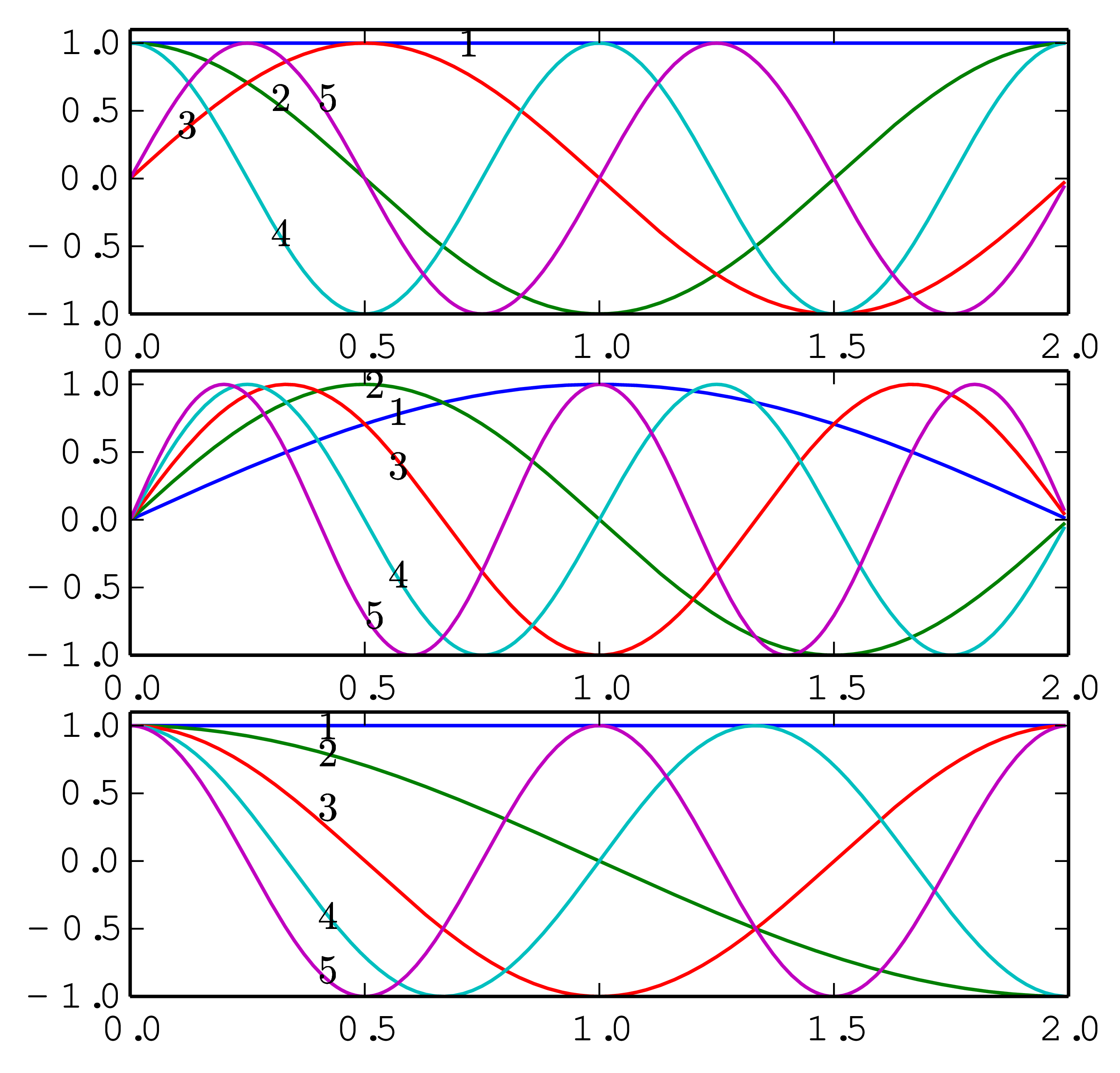 with
with  is a “complete set” in expanding any function in the interval .
A similar conclusion is that the set of cosine functions
is a “complete set” in expanding any function in the interval .
A similar conclusion is that the set of cosine functions  with
with  is a “complete
set” in expanding any function in the
interval . Note that the
argument of the basis functions used in the Fourier expansion differ
from those used in the sine/cosine expansion by a factor of two.
is a “complete
set” in expanding any function in the
interval . Note that the
argument of the basis functions used in the Fourier expansion differ
from those used in the sine/cosine expansion by a factor of two.
The first five basis functions used in Fourier expansion, sine expansion, and cosine expansion are plotted in Fig. 2.
 |
The basis function  used in the Fourier expansion
have the properties
used in the Fourier expansion
have the properties  .
Therefore Fourier expansion works best for function that satisfy
.
Therefore Fourier expansion works best for function that satisfy 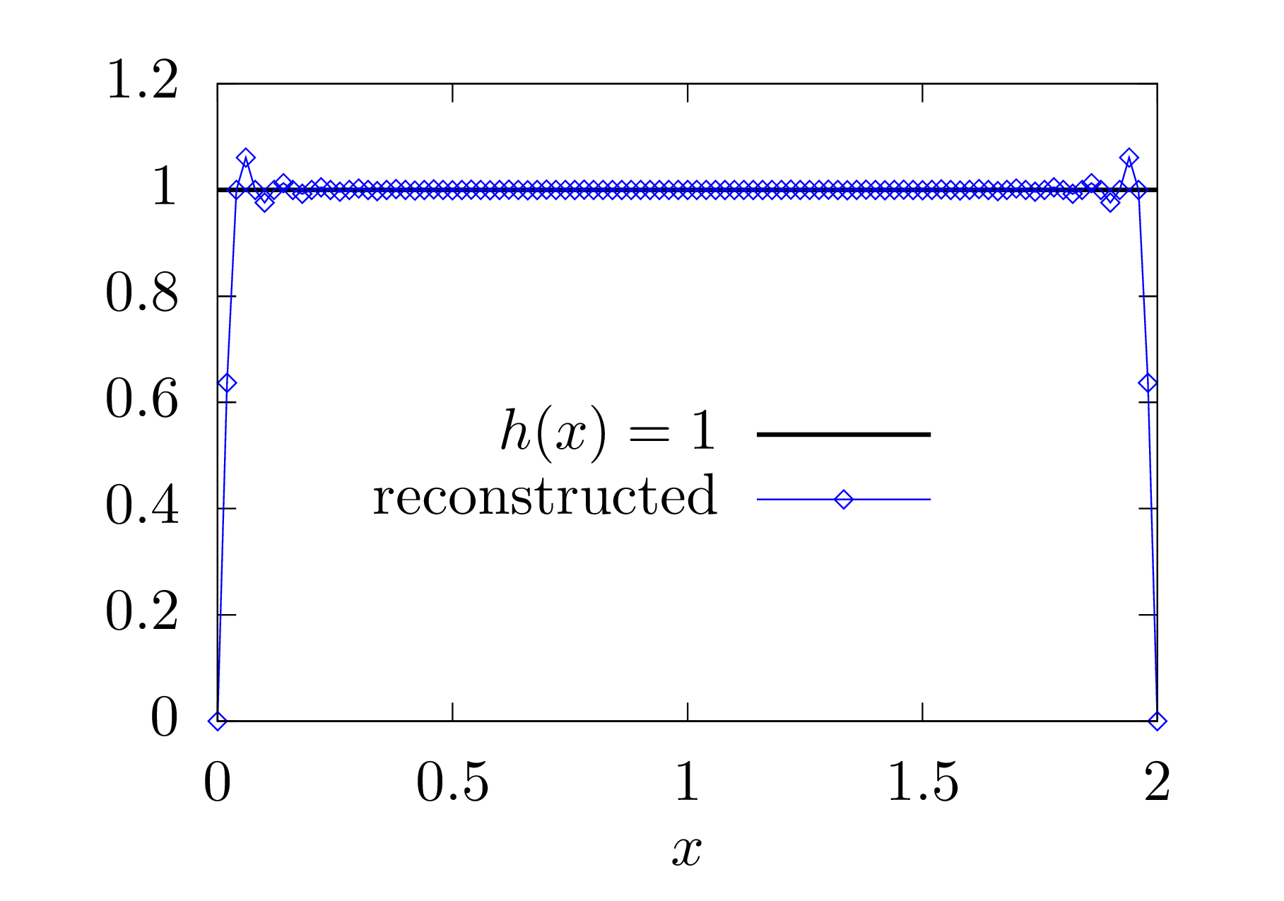 . For a functions that do not
satisfies this condition, i.e., a function with
. For a functions that do not
satisfies this condition, i.e., a function with 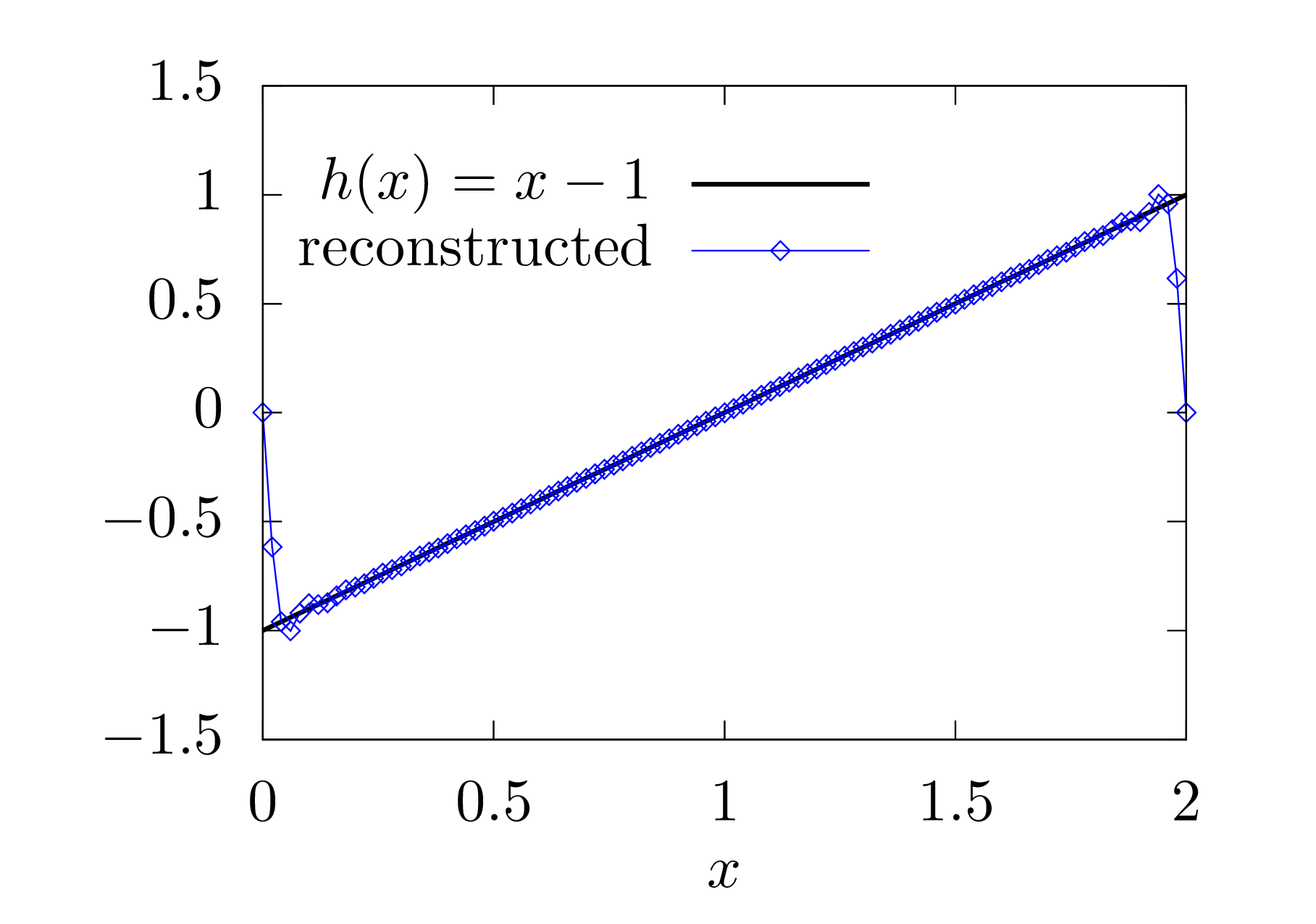 , the function can still be considered as a periodic
function with period but having discontinuity
points at the interval boundary. It is well known that Gibbs
oscillations appear near discontinuity points, which can be inner points
in the interval or at the interval boundaries.
, the function can still be considered as a periodic
function with period but having discontinuity
points at the interval boundary. It is well known that Gibbs
oscillations appear near discontinuity points, which can be inner points
in the interval or at the interval boundaries.
The basis functions used in the sine expansion
have the properties  .
Therefore this expansion works best for functions that satisfy
.
Therefore this expansion works best for functions that satisfy  . For functions that do not
satisfies this condition, there will be Gibbs oscillations near the
boundaries when approximated by using the sine expansion. Examples are
shown in Fig. 3.
. For functions that do not
satisfies this condition, there will be Gibbs oscillations near the
boundaries when approximated by using the sine expansion. Examples are
shown in Fig. 3.
  |
Figure 3. Left: constant function
|
Similarly, the basis functions used in the
cosine expansion have the properties  .
Therefore this expansion works best for functions that satisfy
.
Therefore this expansion works best for functions that satisfy  . For functions that do not
satisfies this condition, there will be Gibbs oscillations near the
boundaries when approximated by using the cosine expansion (to be
verified numerically).
. For functions that do not
satisfies this condition, there will be Gibbs oscillations near the
boundaries when approximated by using the cosine expansion (to be
verified numerically).
Next, let us discuss the sine and cosine transformation. Figure 4 illustrates the grids used in the following discussion.
There are several slightly different types of Discrete Sine Transforms (DST). One form I saw in W. Press's numerical recipe book is given by
 |
(55) |
where  are assumed. This form can be obtained by
replacing DFT's exponential function
are assumed. This form can be obtained by
replacing DFT's exponential function  by
by  . The inverse sine transformation
is given by (I did not derive this, but had numerically verified that
this transform recovers the original data if applied after the sine
transform (55) (code at
/home/yj/project_new/test_space/sine_expansion/t2.f90))
. The inverse sine transformation
is given by (I did not derive this, but had numerically verified that
this transform recovers the original data if applied after the sine
transform (55) (code at
/home/yj/project_new/test_space/sine_expansion/t2.f90))
 |
(56) |
which is identical with the forward sine transformation except for the
normalization factor  . (The
terms of index 0 in both Eq. () and () can be dropped since they are
zero. They are kept to make the representation look more similar to the
DFT, where the index begin from zero.) Replacing
. (The
terms of index 0 in both Eq. () and () can be dropped since they are
zero. They are kept to make the representation look more similar to the
DFT, where the index begin from zero.) Replacing  in Eq. (56) by
  , we obtain the
reconstructing function
, we obtain the
reconstructing function
 |
(57) |
We need a fast method for computing the above DST. All fast methods finally need to make use of the fast method used in the computation of DFT, i.e., FFT. To make use of FFT, we need to define the DST in a way that the DST can be easily connected to the DFT so that FFT can be easily applied. A standard way of making this easy is to define the DST via the DFT of an odd extension of the original data. Next, let us discuss this.
Let us introduce the Discrete Sine Transform (DST) by odd extending a
given real number sequence and then using the DFT of the extended data
to define DST. There are several slightly different ways of odd
extending a given sequence and thus different types of DST. Given a 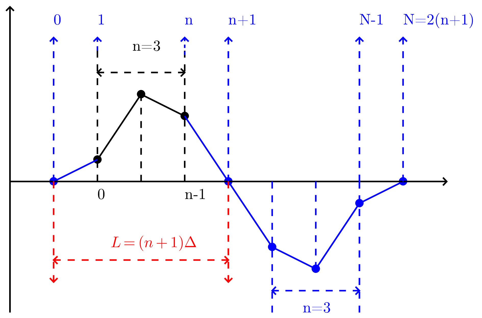 real number sequence
  ,
one frequently adopted odd extension is
,
one frequently adopted odd extension is  .
This odd extension is illustrated in Fig. 5.
.
This odd extension is illustrated in Fig. 5.
As illustrated in Fig. 5, after the old extension, the
total number of points is  with
with  . Then DFT use the
points with index as input. Since the input are
real and odd symmetric sequence, the output of this DFT is an odd
sequence of purely imaginary numbers. Next, let us prove this. The DFT
in this case is given by
. Then DFT use the
points with index as input. Since the input are
real and odd symmetric sequence, the output of this DFT is an odd
sequence of purely imaginary numbers. Next, let us prove this. The DFT
in this case is given by
 |
(58) |
where  is the odd extension of the original data
. For
is the odd extension of the original data
. For  , the relation between and
is given by
, the relation between and
is given by
 |
(59) |
For  , the relation is given
by
, the relation is given
by
 |
(60) |
Noting that  and
and  ,
then expression (58) is written as
,
then expression (58) is written as
 |
(61) |
Using , the above expression
is written as
 |
(62) |
Using the relations (59) and (60) to replace
by ,
the above expression is written
 |
(63) |
Change the definition of the dummy index in the
above summation to make it in the conventional range  , the above expression is written as

Defining  to replace the dummy index in the
second summation, the above expression is written as
to replace the dummy index in the
second summation, the above expression is written as
which is a purely imaginary number. Expression (64) also
indicates  has the following symmetry
 |
(65) |
i.e. odd symmetry. Therefore only half of the data for
with  need to be stored, namely
with
need to be stored, namely
with  . Expression (64)
indicates that
. Expression (64)
indicates that  and
and  are
definitely zero and thus do not need to be stored. Then the remaining
data to be stored are with
are
definitely zero and thus do not need to be stored. Then the remaining
data to be stored are with  , i.e.
  .
Following the convention of making the index of
in the range , we define
.
Following the convention of making the index of
in the range , we define
 . Then
 |
(66) |
with  , which is the index
that we prefer. Finally, the so-called type-I Discrete Sine Transform
(DST-I) is defined based on Eq. (66) via
, which is the index
that we prefer. Finally, the so-called type-I Discrete Sine Transform
(DST-I) is defined based on Eq. (66) via
 |
(67) |
with  . This is the RODFT00
transform defined in the FFTW library.
. This is the RODFT00
transform defined in the FFTW library.
From the above derivation, we know that the DST,  , is related to the DFT, , by
  ,
and thus the meaning of is in principle clear.
Next, let us use the DST to reconstruct the original function from which
the data are sampled. Since DST is only a special case of DFT,
reconstructing the function using DST follows the same procedure used in
DFT. In DFT, the function is reconstructed via Eq. (42)
(changing to the positive exponent convention), i.e.,
,
and thus the meaning of is in principle clear.
Next, let us use the DST to reconstruct the original function from which
the data are sampled. Since DST is only a special case of DFT,
reconstructing the function using DST follows the same procedure used in
DFT. In DFT, the function is reconstructed via Eq. (42)
(changing to the positive exponent convention), i.e.,
 |
(68) |
where is the length of the interval in which the
samplings with are made.
For our present case, i.e., an odd extension of the original data, we have and  and
and  . Then Eq. (68)
is written as
. Then Eq. (68)
is written as
 |
(69) |
Using the odd symmetry of ,
i.e.,  , the above expansion
is written as
, the above expansion
is written as
 |
(70) |
Define  , and note that , then the above expression is
written as
, and note that , then the above expression is
written as
 |
(71) |
i.e.,
 |
(72) |
which is simplified as
 |
(73) |
As a convention, we prefer that the summation index begins from 0 and
ends at  . Then expression (73) is written as

Using the relation between DST and DFT, i.e.,  , the above equation is written as
 |
(74) |
This is the formula for constructing the continuous function using the
DST data. This formula is an expansion over the basis functions  with the DST acting as the
expansion coefficients. Therefore the direct meaning of the DST, , is that they are the expansion
coefficients when using
with the DST acting as the
expansion coefficients. Therefore the direct meaning of the DST, , is that they are the expansion
coefficients when using  as the basis functions
to approximate a function in the domain
as the basis functions
to approximate a function in the domain  .
From Fig. 5, we know that the interval length is given by
.
From Fig. 5, we know that the interval length is given by  ,
where is the uniform spacing between the
original sampling points.
,
where is the uniform spacing between the
original sampling points.
Evaluate the function in Eq. (74) at  with
with  , then we obtain
It can be proved that  in the above equation
exactly recover used in defining the DST . Therefore Eq. (75)
is the Inverse Discrete Sine Transform.
in the above equation
exactly recover used in defining the DST . Therefore Eq. (75)
is the Inverse Discrete Sine Transform.
to be written
The trigonometric identity
 |
(76) |
indicates that nonlinear interaction between two waves of the same frequency generates zero frequency component and its second harmonic. The process of generating of second-harmonic is also called frequency doubling.
Signals that are not band-limited usually contains all frequencies and
thus do not satisfy the condition required by the sampling theorem
(i.e.,  for
for  ).
In this case, for any given data, we can still
calculate its DFT by using Eq. (34). However the results
obtained are meaningful only when approaches
zero as the frequency approaches
).
In this case, for any given data, we can still
calculate its DFT by using Eq. (34). However the results
obtained are meaningful only when approaches
zero as the frequency approaches  from above and
approaches
from above and
approaches  from below, i.e., only when the
results obtained are consistent with the assumption used to obtain the
results (the assumption is that for ). When the results obtained do not satisfy the
above condition, then it indicates that the “aliasing
errors” have contributed to the results. We can reduce the
aliasing errors by increasing the sampling frequency. The aliasing
errors can be reduced but can not be completely removed for a
non-band-limited signal.
from below, i.e., only when the
results obtained are consistent with the assumption used to obtain the
results (the assumption is that for ). When the results obtained do not satisfy the
above condition, then it indicates that the “aliasing
errors” have contributed to the results. We can reduce the
aliasing errors by increasing the sampling frequency. The aliasing
errors can be reduced but can not be completely removed for a
non-band-limited signal.
In signal processing and related disciplines, aliasing is an effect that causes different signals to become indistinguishable (or aliases of one another) when sampled. It also often refers to the distortion or artifact that results when a signal reconstructed from samples is different from the original continuous signal.
An alias is a false lower frequency component that appears in sampled data acquired at too low a sampling rate.
Aliasing errors are hard to detect and almost impossible to remove using software. The solution is to use a high enough sampling rate, or if this is not possible, to use an anti-aliasing filter in front of the analog-to-digital converter (ADC) to eliminate the high frequency components before they get into the data acquisition system.
When a digital image is viewed, a reconstruction is performed by a display or printer device, and by the eyes and the brain. If the image data is processed in some way during sampling or reconstruction, the reconstructed image will differ from the original image, and an alias is seen.
Aliasing can be caused either by the sampling stage or the reconstruction stage; these may be distinguished by calling sampling aliasing (prealiasing) and reconstruction aliasing (postaliasing).
In video or cinematography, temporal aliasing results from the limited frame rate, and causes the wagon-wheel effect, whereby a spoked wheel appears to rotate too slowly or even backwards. Aliasing has changed its apparent frequency of rotation. A reversal of direction can be described as a negative frequency. Temporal aliasing frequencies in video and cinematography are determined by the frame rate of the camera, but the relative intensity of the aliased frequencies is determined by the shutter timing (exposure time) or the use of a temporal aliasing reduction filter during filming.
In the above, we go through the process “Fourier series Fourier transformation DFT”, which corresponds to going from the
discrete case (Fourier series) to the continuous case (Fourier
transformation), and then back to the discrete case (DFT). Since both
Fourier series and DFT are discrete in frequency, it is instructive to
examine the relation between the Fourier coefficient
and the DFT . The Fourier
coefficient of is given by Eq. (93),
i.e.,
Fourier transformation DFT”, which corresponds to going from the
discrete case (Fourier series) to the continuous case (Fourier
transformation), and then back to the discrete case (DFT). Since both
Fourier series and DFT are discrete in frequency, it is instructive to
examine the relation between the Fourier coefficient
and the DFT . The Fourier
coefficient of is given by Eq. (93),
i.e.,
 |
(77) |
which can be equivalently written
 |
(78) |
where  . On the other hand, if
is sampled with sampling rate
. On the other hand, if
is sampled with sampling rate  , then the number of sampling points per period
is
, then the number of sampling points per period
is  . Then the frequency at
which the Fourier transform
. Then the frequency at
which the Fourier transform  is evaluated in
getting the DFT [Eq. (36)] is written
is evaluated in
getting the DFT [Eq. (36)] is written
 |
(79) |
which is identical to the frequency to which the Fourier coefficient
corresponds. Using  in
Eq. (78), we obtain
in
Eq. (78), we obtain
i.e., dividing the DFT by
gives the corresponding Fourier expansion coefficient . We can further use Eqs. (29) and
(30) to recover the Fourier coefficients in terms of
trigonometric functions cosine and sine,
Note that the approximation in Eq. (80) becomes an exact
relation if the largest frequency contained in
is less than .
The Fast Fourier Transform algorithm (FFT) makes the DFT fast enough to solve many real-life problems, which makes FFT be among the top algorithms that have changed the world. The FFT algorithm remained mysterious to me for many years until I read Cooley and Tukey's original paper (An algorithm for the machine calculation of complex Fourier series), which turns out to be a very concise paper and easy to follow.
The DFT is defined by Eq. (34), i.e.,
 |
(82) |
where  . Equations (82)
indicates that the DFT is the multiplication of a transformation matrix
. Equations (82)
indicates that the DFT is the multiplication of a transformation matrix
 with a column vector
  , where the transformation matrix
is symmetric and called DFT matrix. In the matrix form, the DFT is
written as
, where the transformation matrix
is symmetric and called DFT matrix. In the matrix form, the DFT is
written as
 |
(83) |
If directly using the definition in Eq. (83) to compute
DFT, then a matrix multiplication need to be performed, which requires
 operations. Here the powers of
  are assumed to be pre-computed, and we define “an operation”
as a multiplication followed by an addition.
are assumed to be pre-computed, and we define “an operation”
as a multiplication followed by an addition.
The Fast Fourier Transformation (FFT) algorithm manage to reduce the
complexity of computing the DFT from to  by factoring the DFT matrix
into a product of sparse matrices.
by factoring the DFT matrix
into a product of sparse matrices.
Suppose is a composite, i.e.,  . Then the indices in Eq. (82) can
be expressed as
. Then the indices in Eq. (82) can
be expressed as
 |
(84) |
 |
(85) |
Then, one can write
 |
(86) |
Noting that
 |
(87) |
Eq. () is written as
 |
(88) |
where the inner sum over  is independent of
  and can be defined as a new array
 |
(89) |
Then
 |
(90) |
There are elements in the array  , each requiring
  operations, giving a total of
  operation to
obtain . Similarly, it takes
operation to
obtain . Similarly, it takes
 operations to calculate
  from . Therefore, this
two-step algorithm requires a total of
from . Therefore, this
two-step algorithm requires a total of  operations.
Fourier transformationThe Fourier series discussed above indicates that a periodic function is composed of discrete spectrum and is written as
 |
(91) |
where is the period of . The th
term of the above Fourier series corresponds to a harmonic of frequency
 |
(92) |
and the expansion coefficient is given by
 |
(93) |
In terms of  , the coefficient
in Eq. (93) is written
, the coefficient
in Eq. (93) is written
 |
(94) |
In terms of , the Fourier
series in Eq. (91) is written
Note that  is the value of function
  at
at  . Further
note that the interval between and
. Further
note that the interval between and  is . Thus the
above summation is the rectangular formula for numerically calculating
the integration
is . Thus the
above summation is the rectangular formula for numerically calculating
the integration  . Therefore,
equation (95) can be approximately written as
. Therefore,
equation (95) can be approximately written as
 |
(96) |
which will become exact when the interval  ,
i.e.,
,
i.e.,  . Therefore, for the
case , the Fourier series
exactly becomes
. Therefore, for the
case , the Fourier series
exactly becomes
 |
(97) |
where  is given by Eq. (94), i.e.,
 |
(98) |
Note that the function given in Eq. (97)
is proportional to  while the function given in Eq. (98) is proportional to . Since , it is desired to eliminate the
and factors in Eqs. (97) and (98), which can be easily achieved by defining a new function
while the function given in Eq. (98) is proportional to . Since , it is desired to eliminate the
and factors in Eqs. (97) and (98), which can be easily achieved by defining a new function
 |
(99) |
Then equations (97) and (98) are written as
 |
(100) |
 |
(101) |
Equations (100) and (101) are the Fourier transformation pairs discussed in the next section.
As discussed above, the Fourier transformation of a function is given by
 |
(102) |
Once the Fourier transformation  is known, the
original function can be reconstructed via
is known, the
original function can be reconstructed via
 |
(103) |
[Note that the signs in the exponential of Eq. (100) and
(101) are opposite. Which one should be minus or positive
is actually a matter of convention because a trivial variable
substitution  can change the sign between minus
and positive. Proof. In terms of
can change the sign between minus
and positive. Proof. In terms of  ,
Eq. (103) is written
,
Eq. (103) is written
Define
Then Eq. (104) is written
 |
(106) |
The signs in the exponential of Eqs. (105) and (106) are opposite to Eqs. (102) and (103), respectively.]
[Some physicists prefer to use the angular frequency  rather than the frequency
  to represent the
Fourier transformation. Using
to represent the
Fourier transformation. Using  ,
equations. (102) and (103) are written,
respectively, as
,
equations. (102) and (103) are written,
respectively, as
 |
(107) |
 |
(108) |
where we see that the asymmetry between the Fourier transformation and
its inverse is more severe in this representation: besides the
opposite-sign in the exponents, there is also a  factor difference between the Fourier transformation and its inverse.
Whether the factor appears at the forward
transformation or inverse one is actually a matter of convention. The
only requirement is that the product of the two factors in the forward
and inverse transformation is equal to .
To obtain a more symmetric pair, one can adopt a factor
factor difference between the Fourier transformation and its inverse.
Whether the factor appears at the forward
transformation or inverse one is actually a matter of convention. The
only requirement is that the product of the two factors in the forward
and inverse transformation is equal to .
To obtain a more symmetric pair, one can adopt a factor  at both the forward and inverse transformation. The representation in
Eqs. (102) and (103) is adopted in this note.
But we should know how to change to the
representation when needed.]
at both the forward and inverse transformation. The representation in
Eqs. (102) and (103) is adopted in this note.
But we should know how to change to the
representation when needed.]
[
 |
(109) |
]
Next, consider how to numerically compute the Fourier transformation of
a function . A simple way is
to use the rectangle formula to approximate the integration in Eq. (102), i.e.,
 |
(110) |
where and with  . Note Eq. (110) is an
approximation, which will become exact if .
In practice, we can sample only with a nonzero
. Therefore Eq. (110)
is usually an approximation. Do we have some rules to choose a suitable
so that Eq. (110) can become a good
approximation or even an exact relation? This important question is
answered by the sampling theorem, which sates that a suitable to make Eq. (110) exact is given by , where
. Note Eq. (110) is an
approximation, which will become exact if .
In practice, we can sample only with a nonzero
. Therefore Eq. (110)
is usually an approximation. Do we have some rules to choose a suitable
so that Eq. (110) can become a good
approximation or even an exact relation? This important question is
answered by the sampling theorem, which sates that a suitable to make Eq. (110) exact is given by , where  is
the largest frequency contained in (i.e., for
is
the largest frequency contained in (i.e., for  ).
).
In computational and experimental work, we know only a list of values
 sampled at discrete values of
  . Let us suppose that
is sampled with uniform interval between consecutive points:
. Let us suppose that
is sampled with uniform interval between consecutive points:
 |
(111) |
The sampling rate is defined by .
The sampling theorem states that: If the Fourier transformation of
function , , has the following property
 |
(112) |
then sampling with the sampling rate  (i.e., ) will
completely determine , which
is given explicitly by the formula
(i.e., ) will
completely determine , which
is given explicitly by the formula
 |
(113) |
We will not concern us here with the proof of the sampling theorem and
simply start working with Eq. (113) to derive the concrete
expression for the Fourier transformation of . Substituting the expression (113) for
into the Fourier transformation (102),
we obtain the explicit form of the Fourier transformation of :
With the help of Wolfram Mathematica, the integration in Eq. (114) is evaluated analytically, giving
 |
(115) |
Using this, Eq. (114) is written
 |
(116) |
which shows that for , which is consistent with the assumption of
sampling theorem, i.e., has the property given
in Eq. (112). The second line of Eq. (116) is
identical to Eq. (110) except that Eq. (116)
in this case is exact while Eq. (110) is only approximate.
In other words, if , then the
Fourier transformation is exactly given by Eq. (116), where
is the largest frequency contained in (i.e., for ).
Compared with Eq. (1) that uses the trigonometric
functions, Fourier series (15) and (16), which
is expressed in terms of the complex exponential function  , is more compact. The convenience introduced
by the complex exponential function is more obvious when we deal with
multiple-dimensional cases. For example, a two-dimensional function
, is more compact. The convenience introduced
by the complex exponential function is more obvious when we deal with
multiple-dimensional cases. For example, a two-dimensional function  can be expanded as Fourier series about ,
 |
(117) |
where  is the period of
  in direction. The expansion coefficients
  can be further expanded as Fourier series about
  ,
,
 |
(118) |
where  is the period of
in direction, and the coefficients
is the period of
in direction, and the coefficients  is given by
Using Eq. (118) in Eq. (117), we obtain
 |
(120) |
Equations (120) and (119) give the
two-dimensional Fourier series of .
The formula for expanding a real-valued two-dimensional function  in terms of basis functions
  and
and  can be readily recovered from Eqs. (120)
and (119). For notation ease, define
can be readily recovered from Eqs. (120)
and (119). For notation ease, define
 |
(121) |
Then Eq. (120) is written as

Sine is assumed to be real-valued, the imaginary
parts of the above expression will cancel each other. Therefore, the
above expansion is simplified to
This is a compact Fouier expansion for 2D real-valued function.
Furthermore, noting that  term is equal to
  term, the above expansion can be further reduced to
with
 |
(124) |
and the other coefficients given by
 |
(125) |
 |
(126) |
Here the range of  is reduced to
  . In this case, we have an edge case,
  , that needs special treatment. We
see that allowing the index runing from to has the advantage of that there are no edge cases
that needs special treatment.
, that needs special treatment. We
see that allowing the index runing from to has the advantage of that there are no edge cases
that needs special treatment.
We see that the extension of Fourier series from one-dimension case to
two-dimension case is straightforward when expressed in terms of the
complex exponential function .
However, if we use  ,
,  ,
,  ,
and
,
and  as basis functions, the derivation of the
two-dimensional Fourier series of is a little
complicated (product-to-sum trigonometric identities are involved to
simplify the results). Let's see the derivation. A two-dimensional
function can be first expanded as Fourier series
about ,
as basis functions, the derivation of the
two-dimensional Fourier series of is a little
complicated (product-to-sum trigonometric identities are involved to
simplify the results). Let's see the derivation. A two-dimensional
function can be first expanded as Fourier series
about ,
 |
(127) |
(the zero-frequency component is dropped, will take it back later) and
then the two coefficients  and
and  can be further expanded as Fourier series about ,
 |
(128) |
 |
(129) |
(the zero-frequency component is dropped, will take it back later) Substituting Eq. (128) and (129) into Eq. (127), we obtain
Using the product-to-sum trigonometric identities, equation (130) is written

which can be organized as
The coefficients appearing above are written as
 |
(132) |
 |
(133) |
 |
(134) |
 |
(135) |
 |
(136) |
 |
(137) |
Noting that  , and
, and  and
and  , then Eq.
(131) can be written as
, then Eq.
(131) can be written as
 |
|
 |
|
|
 |
 |
The coefficients can be further written as
 |
 |
 |
|
|
|
 |
|
|
|
 |
 |
|
 |
|
|
|
 |
|
|
|
 |
Then comes the drudgery to handle the special cases of  and/or . The final results
are identical to Eqs. (123)-(126). This kind
of derivation is also discussed in my notes on mega code.
and/or . The final results
are identical to Eqs. (123)-(126). This kind
of derivation is also discussed in my notes on mega code.
The following is about a specific FFT subroutine provided by the Numerical recipes book[2]. This is not a general case.
The input and output of the DFT are usually complex numbers. In the
implementation of FFT algorithm provided by Numerical recipes book[2], to avoid using complex numbers, the algorithm adopts the
real number representation of the complex numbers. In this scheme, two
elements of a real number array are used to store one complex number. To
store a complex array “cdata” of length , we will need a real number array
“rdata” of length  .
The first elements of array “rdata” will contain the real
part of “cdata(1)”, the second elements of
“rdata” will contain the imaginary part of
“cdata(1)”, and so on.
.
The first elements of array “rdata” will contain the real
part of “cdata(1)”, the second elements of
“rdata” will contain the imaginary part of
“cdata(1)”, and so on.
To test the correctness of the above statement, I generated a real
number array with length 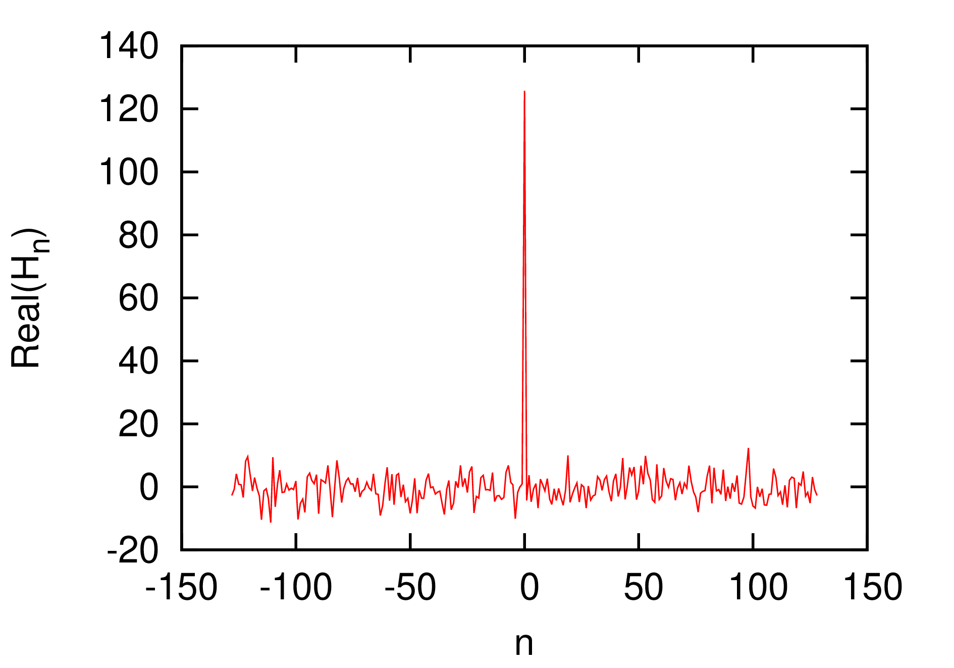 by using a random
generating routine and calculate the DFT of the array with two methods.
The real array generated by the random generator are considered to be a
real number representation of a complex array with length
by using a random
generating routine and calculate the DFT of the array with two methods.
The real array generated by the random generator are considered to be a
real number representation of a complex array with length 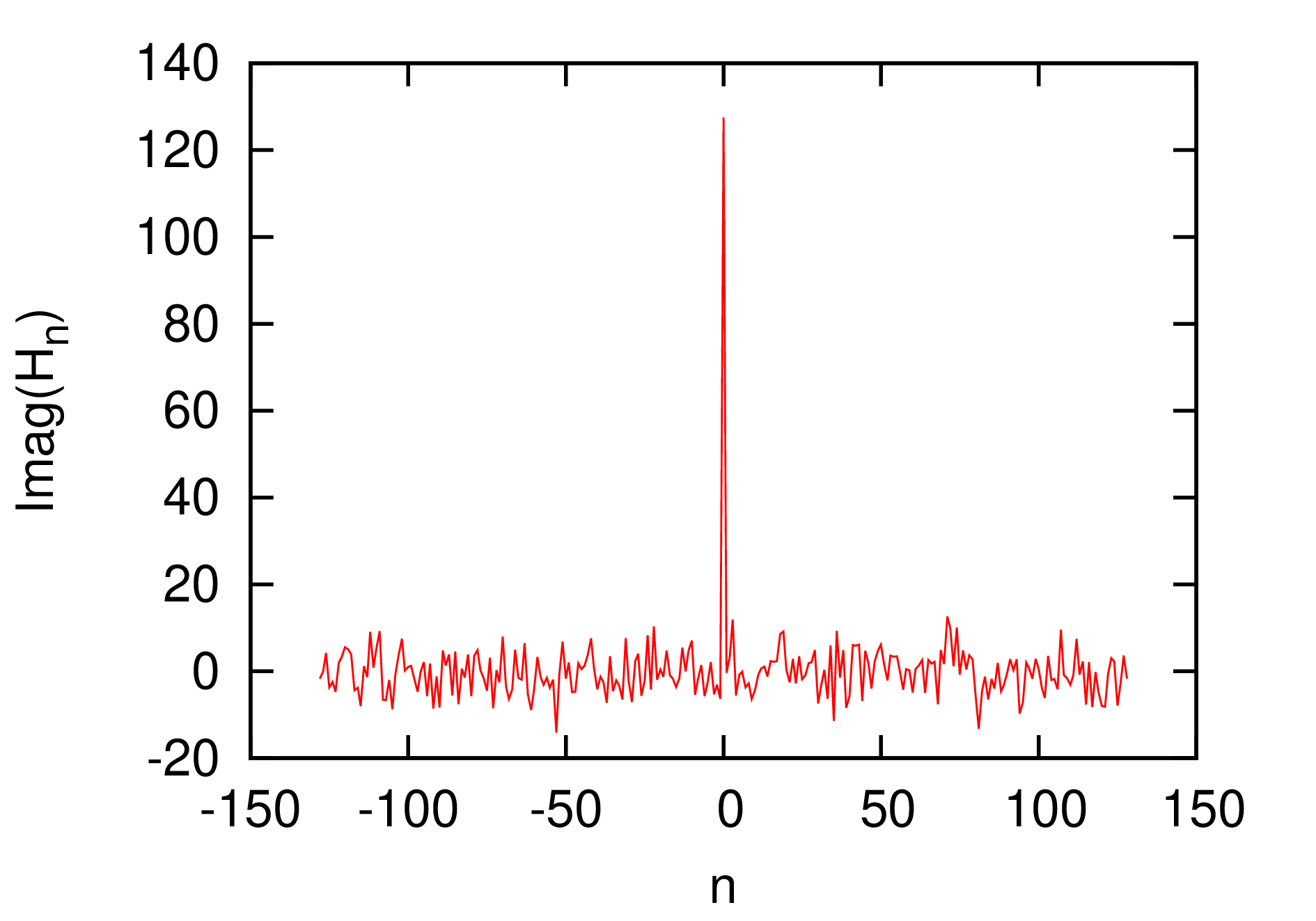 . Using the real array as the input of the FFT
routine (the code in ~/project_new/fft). To check the correctness of my
understanding of the input and output of the FFT, I manually convert the
real number of length to a complex array with
length , and use directly the
summation in Eq. () to calculate the DFT. The output I got is obviously
a complex array with length .
Then I manually convert the complex array to a real number array of
length and plot the output in Fig. 6
with dashed line. The results in Fig. 6 indicates the
results given by the FFT and the naive method used by me agree with each
other well. This proves that my understanding of the input and output of
FFT (especially the storage arrangement) is correct.
. Using the real array as the input of the FFT
routine (the code in ~/project_new/fft). To check the correctness of my
understanding of the input and output of the FFT, I manually convert the
real number of length to a complex array with
length , and use directly the
summation in Eq. () to calculate the DFT. The output I got is obviously
a complex array with length .
Then I manually convert the complex array to a real number array of
length and plot the output in Fig. 6
with dashed line. The results in Fig. 6 indicates the
results given by the FFT and the naive method used by me agree with each
other well. This proves that my understanding of the input and output of
FFT (especially the storage arrangement) is correct.
To clearly show the output of FFT, we recover the real and imaginary part of DFT from the output of FFT and plots the data as a function of their corresponding frequency. The results are given in Fig. 7.
  |
Figure 7. The real (left) and
imaginary (right) part of the discrete Fourier transformation as
a function of the frequency. The point |
Consider the calculation of the following integral:
 |
(141) |
Divide the interval  into
into  uniform sub-intervals and define
 |
(142) |
Then the integration in Eq. (141) can be approximated as
 |
(143) |
Define  with integer and
 . Consider the calculation of
 . Using Eq. (143),
we obtain
. Using Eq. (143),
we obtain
Equation (145) indicates the value of the integration can be obtained by calculating the discrete Fourier
transformation of . However,
as discussed in Ref. [2], equation (145) is
not recommended for practical use because the oscillatory nature of the
integral will make Eq. (145) become systematically
inaccurate as increases. Next, consider a new
method, in which is expanded as
 |
(146) |
Apply the integral operator to both sides of Eq.
(146), we obtain
to both sides of Eq.
(146), we obtain
 |
(147) |
Make the change of variables  in the first
integral and
in the first
integral and  in the second integral, the above
equation is written as
in the second integral, the above
equation is written as
 |
(148) |
Define  and make use of
  , the above equation is written as
 |
(149) |
Define
 |
(150) |
 |
(151) |
Then Eq. (149) is written as
 |
(152) |
|


 is the
period of the signal.
is the
period of the signal.

 with
with  and
and  .
. approximated by using the sine
expansion. Right: linear function
approximated by using the sine
expansion. Right: linear function  approximated by using the sine expansion. Gibbs oscillation
appears near the boundaries, where
approximated by using the sine expansion. Gibbs oscillation
appears near the boundaries, where  (
( for this case). The
expansion coefficients
for this case). The
expansion coefficients  .
. .
.
 and ends at
  .
.
 ).
). ,
, .
. with
with  is the spacing between points.


 corresponds to frequency
  while the point
 corresponds to frequency
  ,
,


