Machine learning

Youjun Hu
yjhu@ipp.cas.cn

July 1, 2024

1 Introduction
2 Neural network
3 Automatic diﬀerentiation
4 misc
5 Least square
6 Logistic regression for binary classiﬁcation
References

1 Introduction

Artiﬁcial intelligence (AI) research has tried many diﬀerent approaches since its founding. In the ﬁrst decades of the 21st century, the AI research is dominated by highly mathematical optimization machine learning (ML), which has proved successful in solving many challenging real life problems.

Many problems in AI can be solved theoretically by searching through many possible solutions: Reasoning can be reduced to performing a search. Simple exhaustive searches are rarely suﬃcient for most real-world problems. The solution, for many problems, is to use ”heuristics” or ”rules of thumb” that prioritize choices in favor of those more likely to reach a goal. A very diﬀerent kind of search came to prominence in the 1990s, based on the mathematical theory of optimization. Modern machine learning is based on these methods. Instead, of using detailed explanations to guide the search, it uses a combination of[1]: (a) general architectures; (b) trying trillions of possibilities, guided by simple ideas (like gradient descent) for improvement; and (c) the ability to recognize progress (by deﬁning a objective function).

I am interested in applying machine learning to problems in computational physics problems that traditional numerical methods can not easily handle either because of its computational costs being too high or its traditional algorithms are too complicated to easily implement.

Enrico Fermi once criticized the complexity of a model (that contains many free parameters) by quoting Johnny von Neumann “With four parameters I can ﬁt an elephant, and with ﬁve I can make him wiggle his trunk”. What Fermi implies is that it is easy to ﬁt existing data and what is important is to have a model with predicting capability (ﬁtting data not seen yet). The artiﬁcial neural network method tackles this diﬃculty by increasing the number of free parameters to millions, with the hope of obtaining predicting capability.

2 Neural network

Neural networks consists of multiple layers of interconnected nodes (neurons), each having a weight for a connection, a bias, and an activation function. Each layer build upon the previous layer. This progression of computations through the network is called forward propagation. Another process called backpropagation uses algorithms which moves backwards through the layers to eﬃciently compute the partial derivatives of the objective function with respect to the weights and biases. Combining the forward and backward propagation, we can calculate errors in predictions and then adjusts the weights and biases using the gradient descent method. This process is called training/learning.

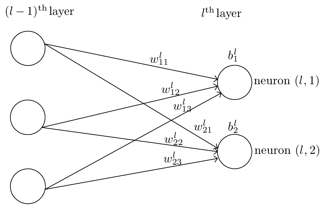
2.1 Node (neuron or unit), weight, bias, and activation

As is shown in Fig. 1, we use w_jk^l to denote the weight for the connection from the k^th neuron in the (l − 1)^th layer to the j^th neuron in the l^th layer. Use b_j^l to denote the bias of the j^th neuron in the l^th layer.

Figure 1: Deﬁnition of layers, neurons, weights, and biases in a neural network. The j^th neuron in the l^th layer is referred to as neuron (l,j)

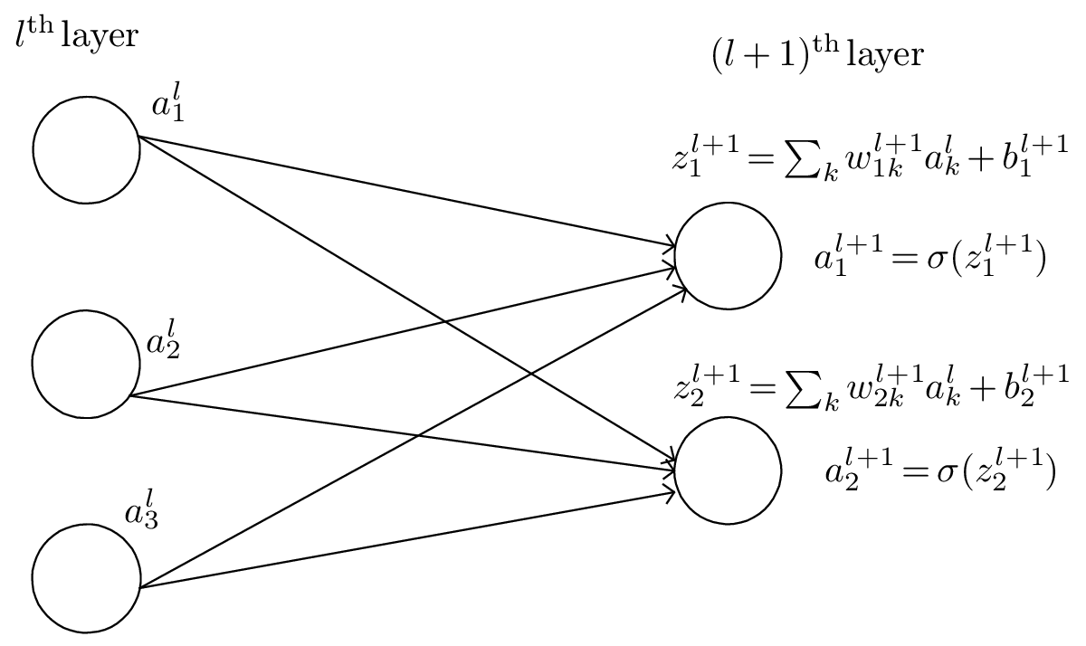
We use a_j^l to denote the output (activation) of the j^th neuron in l^th layer. A neural network model assumes that a_j^l is related to the a^l−1 (output of the previous layer) via

( ) l ∑ l l−1 l aj = σ w jkak + bj , k

(1)

where the summation is over all neurons in the (l − 1)^th layer and σ is a function called activation function which can take various forms, e.g., step function,

{ 1ifz ≥ 0 σ(z) = 0 else ,

(2)

rectiﬁed linear unit (ReLU),

σ (z) = max(0,z),

(3)

and sigmoid (“S”-shaped curve, also called logistic function)

σ(z) =-----1-----. 1 + exp (− z)

(4)

For natation ease, deﬁne z_j^l by

∑ zlj = wljkal−k1 + blj, k

(5)

which can be interpreted as an weighted input to the neuron (l,j), then Eq. (1) is written as

alj = σ (zlj).

(6)

In matrix form, Eq. (5) is written as

zl = wlal−1 + bl,

(7)

where w^l is a J × K matrix, z^l and b^l are column vectors of length J, a^l−1 is a column vector of length K, where J and K are the number of neurons in the l^th layer and (l − 1)^th layer, respectively.

The input layer is where data inputs are provided, and the output layer is where the ﬁnal prediction is made. The input and output layers of a deep neural network are called visible layers. The layers between the input layer and output layer are called hidden layers. Note that the input layer is usually not considered as a layer of the network since it does not involve any computation. In tensorﬂow, layers refer to the computing layers (i.e., hidden layers and the output layer, not including the input layer). The activation function of each layer can be diﬀerent. The activation function of the output layer is often chosen as None, ReLU, logistic/tanh, and is usually diﬀerent from those used in the hidden layers. Here “None” means activation σ(z) = z.

2.2 Objective function

Deﬁne an objective function (can be called loss or cost function depending on contexts) by

C(w,b) ≡ 1-∑ ∥y(x)− aL∥2, 2n x

(8)

where w and b denotes the collection of all weights and biases in the network, n is the total number of training examples x, the summation is over all the training examples, y(x) is the desired output from the network (i.e., correct answer) when x is the input, and a^L is the actual output from the output layer of the network and is a function of w,b, and x. Note that y and a^L are vectors (with number of elements being the number of neurons in the output layer) and ∥…∥ denotes the vector norm. Explicitly writing out the vector norm, Eq. (8) is written as

1 ∑ N∑L C (w, b) ≡ 2n- (yj(x)− aLj )2, x j=1

(9)

where N_L is the number of neurons in the output layer.

The cost function is the average error of the approximate solution away from the desired exact solution. The goal of a learning algorithm is to ﬁnd weights and biases that minimize the cost function. A method of minimizing the cost function over (w,b) is the gradient descent method:

wljk → wljk − η-∂Cl-, ∂w jk

(10)

bl→ bl − η∂C-, j j ∂blj

(11)

where η is called learning rate, which should be positive.

In using the gradient descent method, we need to compute the partial derivatives ∂C∕∂w_jk^l and ∂C∕∂b_j^l. Next we will discuss how to compute them.

2.3 Gradients of objective function

Note that the loss function involves an average over all the training examples. Denote the loss function for a speciﬁc training example by C_x, i.e.,

N∑L Cx = 1 (yj(x)− aLj )2, 2 j=1

(12)

then expression (9) is written as

1 ∑ C = -- Cx, n x

(13)

Then the partial derivatives ∂C∕∂w_jk^l and ∂C∕∂b_j^l can be written as the sum of ∂C_x∕∂w_jk^l and ∂C_x∕∂b_j^l, i.e.,

∂C 1 ∑ ∂C ---l-= -- ---xl-, ∂w jk n x ∂w jk

(14)

∑ ∂Cl = 1- ∂Cxl-. ∂bj n x ∂bj

(15)

The above formulas indicate that, once ∂C_x∕∂w_jk^l and ∂C_x∕∂b_j^l are known, obtaining ∂C∕∂w_jk^l and ∂C∕∂b_j^l is trivial, i.e., just averaging them. Therefore, we will focus on C_x (i.e., the cost function for a ﬁxed training example) and discuss how to compute ∂C_x∕∂w_jk^l and ∂C_x∕∂b_j^l.

In practice, we do not sum over all the training examples. Instead, we average the derivative over a small number (say 16) of training examples (a mini batch) and use these approximate derivatives to advance a step. For the next step, we stochastically change to using a diﬀerent mini batch. This is called stochastic gradient descent (SGD) method.

2.4 Back-propagating algorithm

The cost function C_x is a function of weights and biases of all neurons (the input x and output y(x) are ﬁxed parameters). For a speciﬁc neuron (l,j), its weights and biases enter C_x via the combination z_j^l = ∑ _kw_jk^la_k^l−1 + b_j^l. Then it is useful to deﬁne the following partial derivative:

l ∂Cx δj ≡ ∂zl, j

(16)

where the partial derivative are taken with ﬁxed weights and biases for all neurons except neuron (l,j). Note that the a_k^l−1 appearing in the expression of z_j^l does not depend on w_jk^l or b_j^l. It only depends on the weights and biases in the layers ≤ (l − 1), which are all ﬁxed when taking the derivative in expression (16). δ_j^l deﬁned in expression (16) is often called the error of neuron (l,j).

Using the chain rule, ∂C_x∕∂w_jk^l and ∂C_x∕∂b_j^l can be expressed in terms of δ_j^l:

∂C ∂C ∂zl --xl-= ---xl--jl = δjl, ∂bj ∂zj ∂bj

(17)

and

∂Cx-- ∂Cx--∂zlj- ll−1 ∂wl = ∂zl ∂wl = δjak . jk j jk

(18)

Therefore, if δ_j^l is known, it is trivial to compute the gradients needed in the gradient descent method.

For the output layer (L^th layer), δ_j^l deﬁned in Eq. (16) is written as

∂Cx ∂Cx ∂aLj δLj = ∂zL-= ∂aL-∂zL-. j j j

(19)

The dependence of C_x on a_j^L is explicitly given by Eq. (12), from which the above expression for δ_j^L is written as

L L ′ L δj = (aj − yj(x))σ (zj ).

(20)

Therefore δ_j^L is easy to compute.

Backpropagation is a way of computing δ_j^l for every layer using recurrence relations: the relation between δ^l and δ^l+1. Noting how the error is propagating through the network, we know the following identity:

∂Cx- l ∑ -∂Cx- l+1 ∂zldzJ = ∂zl+1dzj , J j j

(21)

with

l+1 l+1 l dzj = wjJ d(aJ),

(22)

i.e.,

l+1 l+1 ′ l l dzj = wjJ σ(zJ)dzJ.

(23)

Therefore

∂Cx- ∑ -∂Cx- l+1 ′ l ∂zl = ∂zl+1wjJ σ (zJ). J j j

(24)

i.e.,

l ∑ l+1 l+1 ′ l δJ = δj w jJ σ (zJ). j

(25)

Equation (25) gives the recurrence relations of computing δ^l from δ^l+1. This is called the backpropagation algorithm. Eq. (25) can be written in the matrix form:

l l+1 T l+1 ′ l δ = ((w ) δ )⊙ σ (z ),

(26)

where T stands for matrix transpose, ⊙ is the element-wise product.

3 Automatic diﬀerentiation

Automatic diﬀerentiation (autodiﬀ) is a set of techniques for computing derivatives of numeric functions expressed as source code (i.e. the internal mechanism of the function is known). It works by breaking down functions into elementary operations (addition, multiplication, etc.) whose derivatives are known, and then applies the chain rule to compute the derivatives.

Autodiﬀ can be considered as a kind of symbolic diﬀerentiation. The diﬀerence of autodiﬀ from the traditional symbolic diﬀerentiaton is that the goal is not to get a compact formula for humans to understand, but for computers to evaluate. Therefore the ﬁnal result from a autodiﬀ is not an analytical formula, but numerical data. This goal also makes autodiﬀ more eﬃcient since autodiﬀ doses not need to perform some intermedia processes that appear when you use traditional symbolic diﬀerentiation to get a formula and then numerically evaluate the formula.

Autodiﬀ can be better than numerical diﬀerentiation (e.g., ﬁnite diﬀerence) in that it avoid truncation errors. When you are given a black-box function, you can not use autodiﬀ since the internal mechinism of the function is unknown. In this case, the only choice is to use numerical diﬀerentiation.

Autodiﬀ has two main modes: forward and backward. Forward mode computes a single derivative during one pass of the expression tree. The back mode computes all the derivatives in a single pass of the expression tree, avoiding some computational repetition (compared using forward mode to compute all the derivatives sperately). It’s more eﬃcient for functions with many inputs and few outputs, making it ideal for machine learning where we often compute gradients of scalar loss functions with respect to many parameters. Backpropagation is a speciﬁc instance of backward-mode autodiﬀ. Here is a simple Python code implementing autodiﬀ:

Forward:

class Expression:
    def __add__(exp1, exp2):
        return Plus(exp1, exp2)
    def __mul__(exp1, exp2):
        return Multiply(exp1,exp2)
class Variable(Expression):
    def __init__(self,value):
        self.value = value
    def evaluate(self):
        return self.value
    def derive(self, v):
        return 1 if self == v else 0

class Plus(Expression):
    def __init__(self,exp1,exp2):
        self.a = exp1
        self.b = exp2
    def evaluate(self):
        return self.a.evaluate() + self.b.evaluate()
    def derive(self,v):
        return self.a.derive(v) + self.b.derive(v)

class Multiply(Expression):
    def __init__(self,exp1,exp2):
        self.a = exp1
        self.b = exp2
    def evaluate(self):
        return self.a.evaluate() * self.b.evaluate()
    def derive(self, v):
        return (self.a.derive(v)*self.b.evaluate()
               +self.b.derive(v)*self.a.evaluate())

# Example: derivatives of z(x,y) at (x, y) = (2, 3)
x = Variable(2)
y = Variable(3)
z = x * (x + y) + y * y
print(z.derive(x)) # dz/dx,  Output: 7
print(z.derive(y)) # dz/dy,  Output: 8

This simple example illustrates several important concepts:

* Class, subclass, inheritance

* Operator overloading

* Polymorphism

* Recursion

The following is the backward (or reverse) method.

class Expression:
    def __add__(exp1, exp2):
        return Plus(exp1,exp2)
    def __mul__(exp1, exp2):
        return Multiply(exp1, exp2)

class Variable(Expression):
    def __init__(self,value):
        self.value = value
        self.partial = 0
    def evaluate(self):
        return self.value
    def derive(self,seed):
        self.partial += seed

class Plus(Expression):
    def __init__(self,exp1,exp2):
        self.a = exp1
        self.b = exp2
    def evaluate(self):
        return self.a.evaluate() + self.b.evaluate()
    def derive(self,seed):
        self.a.derive(seed)
        self.b.derive(seed)

class Multiply(Expression):
    def __init__(self,exp1,exp2):
        self.a = exp1
        self.b = exp2
    def evaluate(self):
        return self.a.evaluate() * self.b.evaluate()
    def derive(self,seed):
        self.a.derive(seed * self.b.evaluate())
        self.b.derive(seed * self.a.evaluate())

x = Variable(2)
y = Variable(3)
z = x * (x + y) + y * y
z.derive(1)
print(x.partial)  # dz/dx Output:  7
print(y.partial)  # dz/dy Output:  8

Another method is to use dual numbers. Dual number are expressions of the form a + b𝜀, where a and b are real numbers, and 𝜀 is a symbol taken to satisfy 𝜀² = 0 with 𝜀≠0. Using a dual number in the Taylor series, we obtain

∑∞ f(n)(a) n ′ f(a +b𝜀) = n! (b𝜀) = f(a)+ bf (a)𝜀, n=0

(27)

since all terms invovling 𝜀² and greater powers are zero by the deﬁntion of 𝜀. We ﬁnd the coeﬃcient of 𝜀 in the result is the ﬁrst derivative f′(a). This result can be used in computer programs to ﬁnd derivative of a function by deﬁning a class and overloading the basic operators, e.g.

a1 + b1𝜀+ a2 +b2𝜀 = (a1 + a2) +(b1 + b2)𝜀,

(28)

(a1 + b1𝜀)⋆(a2 + b2𝜀) = a1a2 + (a1b2 +a2b1)𝜀.

(29)

Here is a Python code:

class Dual:
    def __init__(self, realPart, infs=0):
        self.realPart = realPart
        self.infs = infs

    def __add__(self, other):
        return Dual(
            self.realPart + other.realPart,
            self.infs + other.infs
        )

    def __mul__(self, other):
        return Dual(
            self.realPart * other.realPart,
            other.realPart * self.infs + self.realPart * other.infs
        )

def f(x, y):
    return x * (x + y) + y * y
x = Dual(2)
y = Dual(3)
epsilon = Dual(0, 1)
a = f(x + epsilon, y)
b = f(x, y + epsilon)
print("dz/dx =", a.infs)  # Output: dz/dx= 7
print("dz/dy =", b.infs)  # Output: dz/dy = 8

4 misc

5 Least square

In the least square method, the loss function is deﬁned as

∑n 2 L = |ˆy(xi)− yi|, i=1

(30)

where (x_i) is the output of the model for the input x_i, n is the number of data points.

In the most general case, each data point considers of multiple independent variables and multiple dependent variables (x,y). In simple cases, each data point has one independent variable and one dependent variable. For example, a data set consists of n data-points (x_i,y_i), i = 1, …, n, where x_i is an independent variable and y_i is a dependent variable whose value is found by observation. The model function has the form y(x) = f(x,β), where m adjustable parameters are held in the vector β. A least squar model is called linear if the model comprises a linear combination of the parameters, i.e.,

m∑ f (x,β) = βjφj(x ), j=1

(31)

where φ_j(x) are basis functions chosen. Letting X_ij = φ_j(x_i), then the model prediction for input x_i can be written as

m f ≡ f(x ,β ) = ∑ X β . i i j=1 ij j

(32)

For n data points, the above can be written in matrix form:

f = Xβ,

(33)

where f = (f₁,…f_n)^T.

For linear least-square ﬁtting, we can solve the “normal equation” to get the ﬁtting coeﬃcients. Alternatively, one can use iterative methods, e.g., the gradient descent method, to minimize the mean square error over the coeﬃcients. The following is a complete example in Python:

import numpy as np
import matplotlib.pyplot as plt
class Linear_Regression:
    def __init__(self):
            self.b = [0, 0]

    def predict(self, X):
            Y_pred = self.b[0] + self.b[1]*X
            return Y_pred

    def update_coeffs(self, X, Y, learning_rate):
            Y_pred = self.predict(X)
            m = len(Y)
            self.b[0] = self.b[0] - (learning_rate * ((1/m) *
                                                      np.sum(Y_pred - Y)))
            self.b[1] = self.b[1] - (learning_rate * ((1/m) *
                                                      np.sum((Y_pred - Y) * X)))

regressor = Linear_Regression()
Nd=11
X = np.array([i for i in range(Nd)])
Y = np.array([2*i for i in range(Nd)]) + np.random.uniform(high=5.0,size=Nd)
fig, ax = plt.subplots()
ax.plot(X,Y, ’k.’,label=’data’)
Y_pred = regressor.predict(X)
ax.plot(X, Y_pred, label=’Initial fit line’)

learning_rate = 0.01
i = 0
while i<100:
    regressor.update_coeffs(X,Y,learning_rate)
    i = i+1

Y_pred = regressor.predict(X)
ax.plot(X, Y_pred, ’b-’,label=’Final Fit Line’)
ax.legend()
plt.show()

The loss function is deﬁned by the mean square error, which is not directly used in the above code. Only the partial derivatives of the loss function is directly used.

6 Logistic regression for binary classiﬁcation

Hypothesis function (the model): Denote the output of the model by ŷ, which is given by

ˆy = σ(z),

(34)

where z = w ⋅ x + b and σ is the sigmoid function given by Eq. (4). The model is nonlinear in the unknowns w and b.

The loss function is chosen as

1 m∑ L = − m- [yilog(ˆyi)+ (1 − yi)log(1− ˆyi)], i=1

(35)

where y_i is the correct answer of the ith training example (y_i can take only two values, 0 or 1). The value of y^i is interpreted as the probability of y being 1.

Because the model function is nonlinear and the loss function is complicated, there is usually no closed-form solution that minimizes the loss function. Iterative methods, such as gradient descent, are needed to solve for w and b. The partial derivatives needed in the gradient desent method can be written as

[ ] ∂L- = −-1 ∑ y 1σ′(z)x − (1 − y)--1---σ′(z)x ∂w m i iˆyi i i (1− ˆyi) i 1 ∑ {[ 1 1 ] } = −-- yi--− (1− yi)-------σ ′(z)xi m i {[ ˆyi ] (1 −}ˆyi) -1 ∑ --yi −y^i ′ = −m ˆyi(1− ˆyi) σ (z)xi ∑i {[ ] } = −-1 --yi −y^i σ(1− σ)xi m i ˆyi(1− ˆyi) 1 ∑ {[ yi −y^i ] } = −m- ˆy-(1−-ˆy-) ˆyi(1− yˆi)xi i i i = −-1 ∑ [(yi − ^yi)xi] (36) m i

Using

dσ- -----1------- 2 dz = (1 + exp(− z))2 exp(− z) = σ exp(− z) = σ(1− σ)

(37)

The above formula is simpliﬁed as

{ [ ] } ∂L- = − 1-∑ -yi−y^i- σ(1− σ )xi ∂w m1 ∑ i{ [ˆyi(y1−−y ˆy^i)] } = − m-∑ i ˆyi(i1−i ˆyi) ˆyi(1− ˆyi)xi = − 1m- i[(yi − y^i)xi]

(38)

Similary, we obtain

∂L-= − 1-∑ (yi − ^yi). ∂w m i

(39)

References

[1] Michael A Nielsen. Neural networks and deep learning, volume 25. Determination Press: http://neuralnetworksanddeeplearning.com/, 2015.