EAST Tokamak equilibrium

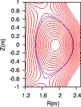
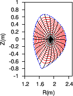
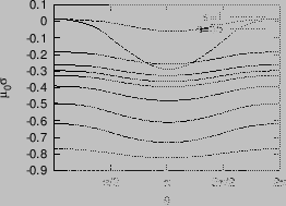
The tokamak equilibrium used in this paper is reconstructed by EFIT code by using the information of profiles measured in EAST experiment[9]. The shape of flux surfaces within the last-closed-flux surface (LCFS) are plotted in Fig. 11, where $\theta = \ensuremath{\operatorname{const}}$ curves are also plotted. In the paper, I said that the equilibrium was a double-null configuration with the LCFS connected to the lower X point. This is wrong. The configuration with the LCFS connected to the lower X point should be called lower single null configuration. The double-null configuration is a configuration with LCFS connected to both the lower and upper X points. In practice, if the spacial seperation between the flux surface connected to the low X point and the flux surface connected to the upper X point, $\ensuremath{\operatorname{dRsep}}$, is smaller than a value (e.g. 1cm), the configuration can be considered as a double null configuration, where $\ensuremath{\operatorname{dRsep}}$ is the spacial separation between the two flux surfaces on the low-field side of the midplane.

Figure 11: Grid points (the intersecting points of two curves in the figure) corresponding to uniform poloidal flux and uniform poloidal arc length for EAST discharge #38300 at 3.9s (G-file name: g038300.03900, which was provided by Dr. Guoqiang Li).

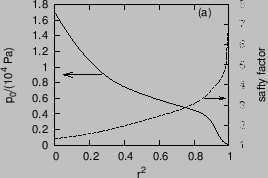
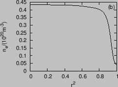
The profiles of safety factor, pressure, and electron number density are plotted in Fig. 12.

Figure 12: Safety factor and pressure (a), toroidal field function (b), and electron number density (c) as a function of the radial coordinate for EAST discharge #38300 at 3.9s (G-eqdsk filename g038300.03900).

The mass density $\rho_0$ is calculated from $\rho_0 = m_i n_i$, where $m_i$ is the mass of the main ions (deuterium ions in this discharge), $n_i$ is the number density of the ions, which is inferred from $n_e$ by using the neutral condition $n_i = n_e$ (impurity ions are neglected).

Figure 13: Normal and geodesic magnetic curvature as a function of the poloidal angle. Different lines in the figure correspond to different magnetic surfaces.

Figure 14: Negative local magnetic shear $S$ as a function of the poloidal angle. The different lines correspond to different magnetic surfaces. The equilibrium is for EAST shot #38300 at 3.9s.

Figure 15: ${\textmu }_0 \sigma$ as a function of the poloidal angle. The different lines correspond to the values of ${\textmu }_0 \sigma$ on different magnetic surfaces