 is
governed by the momentum equation
is
governed by the momentum equation
|
Abstract
This note discusses the linear ideal magnetohydrodynamic (MHD) theory of tokamak plasmas. This note also serves as a document for the GTAW code (General Tokamak Alfvén Waves code), which is a Fortran code calculating Alfven eigenmodes in realistic tokamak geometries.
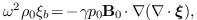
The time evolution of the fluid velocity is
governed by the momentum equation
 |
(1) |
where  ,
,  ,
,  ,
,
 ,
,  , and
, and  are mass density, charge density, thermal pressure, current density,
electric field, and magnetic field, respectively. The time evolution of
the mass density is governed by the mass
continuity equation
are mass density, charge density, thermal pressure, current density,
electric field, and magnetic field, respectively. The time evolution of
the mass density is governed by the mass
continuity equation
 |
(2) |
The time evolution equation for pressure is
given by the equation of state
 |
(3) |
where  is the ratio of specific heats. The time
evolution of is given by Faraday's law
is the ratio of specific heats. The time
evolution of is given by Faraday's law
 |
(4) |
The current density can be considered as a
derived quantity, which is defined through Ampere's law (the
displacement current being neglected)
 |
(5) |
The electric field is considered to be a derived
quantity, which is defined through Ohm's law
 |
(6) |
The charge density can be considered to be a
derived quantity, which is defined through Poisson's equation,
 |
(7) |
The above equations constitute a closed set of equations for the time
evolution of four quantities, namely, , , , and (the
electric field , current density , and charge density are eliminated
by using Eqs. (5), (6), and (6)).
In addition, there is an equation governing the spatial structure of the
magnetic field, namely
 |
(8) |
In summary, the MHD equations can be categorized into three groups of equations, namely[1],
Evolution equations for base quantities ,
, , and :


 ,
,
 ,
,
Equation of constraint:  .
.
Definitions: (i.e., they are considered to be derived quantities.)
 ,
,
 ,
,
 .
.
The electrical field term  in the momentum
equation (1) is usually neglected because this term is
usually much smaller than other terms for low-frequency phenomena in
tokamak plasmas (quasi-neutral approximation).
in the momentum
equation (1) is usually neglected because this term is
usually much smaller than other terms for low-frequency phenomena in
tokamak plasmas (quasi-neutral approximation).
It is well known that the divergence of Faraday's law (4) is written
 |
(9) |
which implies that will hold in later time if it
is satisfied at the initial time.
Because the displacement current is neglected in Ampere's law, the divergence of Ampere's law is written
 |
(10) |
On the other hand, the charge density is defined through Poisson's equation, Eq. (7), i.e.,

which indicates that the charge density is
usually time dependent, i.e.,  . Therefore the
charge conservation is not guaranteed in this framework. This
inconsistency is obviously due to the fact that we neglect the
displacement current
. Therefore the
charge conservation is not guaranteed in this framework. This
inconsistency is obviously due to the fact that we neglect the
displacement current  in Ampere's law. Since, for
low frequency phenomena, the displacement current
term is usually much smaller than the the conducting current , neglecting the displacement current term induces only
small errors in calculating by using Eq. (5).
in Ampere's law. Since, for
low frequency phenomena, the displacement current
term is usually much smaller than the the conducting current , neglecting the displacement current term induces only
small errors in calculating by using Eq. (5).
Referece [2] gives a clear derivation of the generalized Ohm's law, which takes the following form
 |
(12) |
where the first term on the right-hand side is called the “Hall term”, the second term is the electron pressure term, and the third term is called the “electron inertia term” since it is proportional to the mass of electrons.
Note that both and are
the first-order moments, with being the weighted
sum of the first-order moment of electrons and ions while being the difference between them. The generalized Ohm's
law is actually the difference between the electrons and ions
first-order moment equations. The generalized Ohm's law is an equation
that governs the time evolution of . Also note
that Ampere's law, with the displacement current retained, is an
equation governing the time evolution of .
However, in the approximation of the resistive MHD, the time derivative
term is dropped in Ampere's law and and  is dropped in Ohm's law. In this approximation, Ohm's
law is directly solved to determine and Ampere's
law is directly solved to determine .
is dropped in Ohm's law. In this approximation, Ohm's
law is directly solved to determine and Ampere's
law is directly solved to determine .
from equation of state
The equation of state (3) involves three physical
quantities, namely , , and
. It turns out that the continuity equation can
be used in the equation to eliminate . The
equation of state
 |
(13) |
can be written as
 |
(14) |
which simplifies to
 |
(15) |
Expand the total derivative, giving
 |
(16) |
Using the mass continuity equation to eliminate
in the above equation gives
 |
(17) |
This equation governs the time evolution of the pressure. A way to
memorize this equation is that, if  , the equation
will take the same form as a continuity equation, i.e.,
, the equation
will take the same form as a continuity equation, i.e.,
 |
(18) |
For the convenience of reference, the MHD equations discussed above are
summarized here. The time evolution of the four quantities, namely , , ,
and , are governed respectively by the following
four equations:
 |
(19) |
 |
(20) |
 |
(21) |
 |
(22) |
Note that only Eq. (19) involves the resistivity  . When
  , the above system is called
ideal MHD equations.
, the above system is called
ideal MHD equations.
Next, consider the linearized version of the ideal MHD equations. Use
 ,
,  ,
,  ,
and
,
and  to denote the equilibrium fluid velocity,
magnetic field, plasma pressure, and mass density, respectively. Use
to denote the equilibrium fluid velocity,
magnetic field, plasma pressure, and mass density, respectively. Use
 ,
,  ,
,  ,
and
,
and  to denote the perturbed fluid velocity,
magnetic field, plasma pressure, and mass density, respectively.
Consider only the case that there is no equilibrium flow, i.e.,
to denote the perturbed fluid velocity,
magnetic field, plasma pressure, and mass density, respectively.
Consider only the case that there is no equilibrium flow, i.e.,  . From Eq. (21), the linearized equation
for the time evolution of the perturbed pressure is written
. From Eq. (21), the linearized equation
for the time evolution of the perturbed pressure is written
 |
(23) |
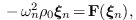
The linearized momentum equation is written
 |
(24) |
The linearized induction equation is written
 |
(25) |
These three equations constitute a closed system for ,
, and . Note that the
linearized equation for the perturbed mass density
 |
(26) |
is not needed when solving the system of equations (23)-(25) because does not appear in
equations (23)-(25).

In dealing with the linear case of MHD theory, it is convenient to
introduce the plasma displacement vector  , which
is defined through the following equation
, which
is defined through the following equation
 |
(27) |
Using the definition of and the fact that the
equilibrium quantities are independent of time, the linearized induction
equation (25) is written
 |
(28) |
Similarly, the equation for the perturbed pressure [Eq. (23)] is written
 |
(29) |
In terms of the displacement vector, the linearized momentum equation (24) is written
 |
(30) |
Equations (28), (29), and (30)
constitute a closed system for , ,
and .
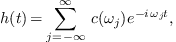
A general perturbation can be written
 |
(31) |
where the coefficient  is given by the Fourier
transformation of
is given by the Fourier
transformation of  , i.e.,
 |
(32) |
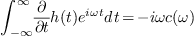
Using the definition of the Fourier transformtion, it is ready to prove that
 |
(33) |
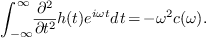
and
 |
(34) |
Performing Fourier transformation (in time) on both sides of the the linearized momentum equation (30) and noting that the equilibrium quantities are all independent of time, we obtain
 |
(35) |
where use has been made of the property in Eq. (34). Similarly, the Fourier transformation of the equations of state (29) is written
 |
(36) |
and the Fourier transformation of Faraday's law (28) is written
 |
(37) |
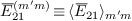
Equations (35)-(37) agree with Eqs. (12)-(14)
in Cheng's paper[3]. They constitute a closed set of
equations for  ,
,  , and
, and  . In the next section, for notation ease, the hat on
, , and
will be omitted, with the understanding that they are the Fourier
transformations of the corresponding quantities.
. In the next section, for notation ease, the hat on
, , and
will be omitted, with the understanding that they are the Fourier
transformations of the corresponding quantities.
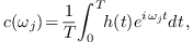
In dealing with eigenmodes, we ususally encounter discrete frequency
perturbations, i.e., is periodic function of
 so that they contian only discrete frequency
components. In this case, the inverse Fourier transformtion in Eq. (31) is replaced by the Fourier series, i.e.,
so that they contian only discrete frequency
components. In this case, the inverse Fourier transformtion in Eq. (31) is replaced by the Fourier series, i.e.,
 |
(38) |
where the coefficients  are given by
 |
(39) |
with  and
and  being the
period of ( is larger
enough so that
being the
period of ( is larger
enough so that  is very small compared with
frequency we are interested). The relation between
and given by Eqs. (33) and (34) also applies to the relation between
and
is very small compared with
frequency we are interested). The relation between
and given by Eqs. (33) and (34) also applies to the relation between
and  , i.e.,
 |
(40) |
and
 |
(41) |
Using the transformtion given by Eq. (39) on Eqs. (28), (29), and (30), respectively, we obtain the same equation as Eqs. (35)-(37).
A general perturbation is given by Eq. (31), which is
composed of infinit single-frequency perturbation of the form  . It is obvious that a general perturbation can also be
considered to be composed of single frequency perturbation of the form
. It is obvious that a general perturbation can also be
considered to be composed of single frequency perturbation of the form
 |
(42) |
In this case the range of  is limited in
  . Because a physical quanty is always a real function,
 in the above should be a real function. It is
ready to prove that the Fourier transformation of
has the following symmetry in frequency domain:
in the above should be a real function. It is
ready to prove that the Fourier transformation of
has the following symmetry in frequency domain:
 |
(43) |
Uisng this, the expression (42) is written

Writing  , where
  and
and  are real numbers, then the above expression is
written as
are real numbers, then the above expression is
written as

Using expression (45), the Fourier transformation is written
 |
(46) |
If  satisfies the eigenmode equations (35)-(37), then it is ready to verify that
  is also a solution to the equations. Then Eq. (43) implies
that
is also a solution to the equations. Then Eq. (43) implies
that  is also a slution to the equations.
Therefore
is also a slution to the equations.
Therefore  , i.e.,
  , is a
solution to the linear equations (28), (29),
and (30). This tell us how to construct a real (physical)
eigenmode from the complex funtion , i.e., the
real part of is a physical eigenmode. Note that
it is the real part of , instead of the real part
of , that is a physical eigenmode.
, is a
solution to the linear equations (28), (29),
and (30). This tell us how to construct a real (physical)
eigenmode from the complex funtion , i.e., the
real part of is a physical eigenmode. Note that
it is the real part of , instead of the real part
of , that is a physical eigenmode.
Note that is a real number by the definition of
Fourier transformation. However, strictly speaking, the above Fourier
transformation should be replaced by Laplace transformation. In this
case, is a complex number. In the following, we
will assume that we are using Laplace transformation, instead of Fourier
transformation. In the following section, we will prove that the
eigenvalue  of the ideal MHD system must be a
real number.
of the ideal MHD system must be a
real number.
Using Eqs. (36) and (37) to eliminate and from Eq. (35),
we obtain
 |
(47) |
where  , the linear force operator, is given by
 |
(48) |
It can be proved that the linear force operator
is self-adjoint (or Hermitian) (I have never proven this), i.e., for any
two general functions  and
and  that satisfy the same boundary condition, we have
 |
(49) |
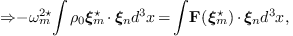
As a consequence of the self-adjointness, the eigenvalue, , must be a real number. [Proof: Taking the complex
conjugate of Eq. (47), we obtain
 |
(50) |
Note that the expression of  given in Eq. (48) have the property
  , Using this,
equation (50) is written
, Using this,
equation (50) is written
 |
(51) |
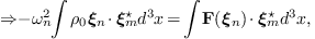
Taking the scalar product of both sides of the above equation with and integrating over the entire volume of the system,
gives
 |
(52) |
Using the self-ajointness of  , the above equation
is written
, the above equation
is written
 |
(53) |
 |
(54) |
 |
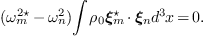
(55) |
Since  is non-zero for any non-trivial
eigenfunction, it follows from Eq. (55) that
is non-zero for any non-trivial
eigenfunction, it follows from Eq. (55) that  , i.e., must be a real number,
which implies that is either purely real or
purely imaginary.] It can also be proved that two eigenfunctions of the
Hermitian operator corresponding to different eigenvalues are orthogonal
to each other. [Proof:
, i.e., must be a real number,
which implies that is either purely real or
purely imaginary.] It can also be proved that two eigenfunctions of the
Hermitian operator corresponding to different eigenvalues are orthogonal
to each other. [Proof:
 |
(56) |
 |
(57) |
Taking the scalar product of both sides of Eq. (56) with
 and integrating over the entire volume of the
system, gives
and integrating over the entire volume of the
system, gives
 |
(58) |
Taking the scalar product of both sides of Eq. (57) with
 and integrating over the entire volume of the
system, gives
and integrating over the entire volume of the
system, gives
 |
(59) |
Combining the above two equations, we obtain

Using the self-ajointness of , we know the
right-hand side of Eq. (59) is zero. Thus Eq. (59)
is written
 |
(61) |
Using  , the above equation is written
 |
(62) |
Since we assume  , the above equation reduces to
 |
(63) |
i.e., and are orthogonal
to each other.]
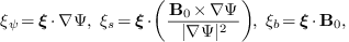
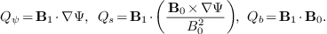
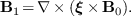
Next, we consider the form of the linearized MHD equations in toroidal devices (e.g. tokamak). In these devices, there exist magnetic surfaces. The motion of plasma along the surface and perpendicular to the surface are very different. Thus, it is useful to decompose the perturbed quantities into components lying on the surface and perpendicular to the surface. Following Ref. [3, 4], we write the displacement vector and perturbed magnetic field as
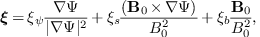 |
(64) |
and
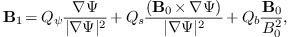 |
(65) |
where  is the poloidal magnetic flux function
appearing in the GS equation (
is the poloidal magnetic flux function
appearing in the GS equation ( ). (In deriving the
eigenmode equation, we do not need the specific definition of . What we need is only that
). (In deriving the
eigenmode equation, we do not need the specific definition of . What we need is only that  is a
vector in the direction of
is a
vector in the direction of  and thus is perpendicular to both and
  ). Taking scalar product of the above two equations
with ,
). Taking scalar product of the above two equations
with ,  , and , respectively, we obtain
 |
(66) |
 |
(67) |
Next, we derive the component equations for the induction equation (37) and momentum equation (35). The derivation is straightforward but tedious. Those who are not interested in these details can skip them and read directly Sec. 3.7 for the final form of the component equations.
component of
induction equationThe induction equation is given by Eq. (37), i.e.,
 |
(68) |
Next, consider the component of the above
equation. Taking scalar product of the above equation with , we obtain
 |
(69) |
 |
(70) |
 |
(71) |
 |
(72) |
 |
(73) |
 |
(74) |
 |
(75) |
 |
(76) |
 |
(77) |
 |
(78) |
Excluding  terms, the terms on the right hand
side (r.h.s) of the above equation can be written
terms, the terms on the right hand
side (r.h.s) of the above equation can be written
Using  , we obtain


The r.h.s of the above equation is exactly the term appearing on the right-hand side of Eq. (79). Thus we obtain
 |
(82) |
which agrees with Eq. (20) in Cheng's paper[3].
 component of
induction equation
component of
induction equation
The component of the induction equation is given
by
 |
(83) |
which can be further written as
where
 |
(85) |
is the negative local magnetic shear. Using  ,
equation (84) is written as
,
equation (84) is written as
 |
(86) |
 |
(87) |
Eq. (87) agrees with Eq. (21) in Cheng's paper[3].
 component of
induction equation
component of
induction equation
The component of the induction equation in the direction of is written as
 |
(88) |
 |
(89) |
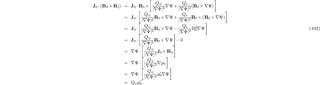
The term on right-hand side of the above equation is written as
Using this, the right-hand side of Eq. (89) is written as
Before we try to simplify the above equation, we derive the expression
for the divergence of , which is written as

It can be proved that the fourth term of the above equation can be written as (refer to (9.8) for the proof)

Then Eq. (93) is written as
 |
(95) |
Eq. (95) agrees with Eq. (23) in Cheng's paper, but a  factor is missed in the fourth term of Cheng's
equation[3]. Using Eq. (95), Eq. (92)
is written as
factor is missed in the fourth term of Cheng's
equation[3]. Using Eq. (95), Eq. (92)
is written as
 |
(96) |
It can be proved that
 |
(97) |
(Refer to Sec. 9.10 for the proof.) Then Eq. (96) is written as
 |
(98) |
and the component of the induction equation in the direction of [Eq. (89)] is finally written as
 |
(99) |
Eq. (99) agrees with Eq. (22) in Cheng's paper[3].
The three components of the linearized momentum equation can be obtained
by taking scalar product of Eq. (35) with ,
 , and , respectively. We
first consider the component of the momentum
equation, which is written as
, and , respectively. We
first consider the component of the momentum
equation, which is written as
 |
(100) |
i.e.,
 |
(101) |
The last term on the right-hand side of Eq. (101) can be written as
where  . Using Eq. (82), i.e.,
  , the above equation is written as
 |
(103) |
Substituting Eq. (103) into Eq. (101) gives
 |
(104) |
Using  in the above equation gives
 |
(105) |
which agrees with Eq. (19) in Cheng's paper[3].
component of
momentum equation
Next we consider the radial component of the momentum equation. Taking
scalar product of the momentum equation with , we
obtain
 |
(106) |
After some algebra (the details are given in Sec. (9.5)), Eq. (106) is written

where
 |
(108) |
and  is the magnetic field curvature with
  the unit vector along equilibrium magnetic field.
Equation (107) agrees with Eq. (17) in Cheng's paper[3]. In passing, let us examine the physical meaning of
the unit vector along equilibrium magnetic field.
Equation (107) agrees with Eq. (17) in Cheng's paper[3]. In passing, let us examine the physical meaning of  defined by (108). In linear
approximation, we have
defined by (108). In linear
approximation, we have

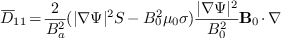
This indicates the perturbation in the square of the magnetic strength
is  . Therefore, the perturbation in magnetic
pressure is written
. Therefore, the perturbation in magnetic
pressure is written
 |
(110) |
which indicate defined by Eq. (108)
is the total perturbation in the thermal and magnetic pressure.
component of
momentum equation
The component of the linearized momentum
equation is written
 |
(111) |
The last term of Eq. (111) is written
Using Eq. (337), i.e.,
 |
(113) |
the second last term on the right-hand side of Eq. (111) is written
The term  in the above equation is written as


Gathering terms involving  , excluding the first
term, in expression (115) gives
, excluding the first
term, in expression (115) gives

which can be proved to be zero (refer to Sec. 9.6 for the
proof). Gathering terms involving  in expression
(115) gives
in expression
(115) gives

It can be proved that the second term of the above expression is equal
to  (refer to Sec. 9.9 for details).
Thus, from Eq. (114), we obtain
(refer to Sec. 9.9 for details).
Thus, from Eq. (114), we obtain
 |
(117) |
Using Eqs. (112) and (117) in Eq. (111) yields
 |
(118) |
Using  , the above equation can be arranged as
 |
(119) |
which agrees with Eq. (18) in Cheng's paper[3].
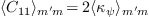
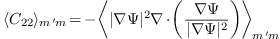
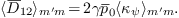
For the ease of reference, Eqs. (29), (82), (87), (99), (105), (76), and (119) are repeated here:
 |
(120) |
 |
(121) |
 |
(122) |
 |
(123) |

 |
(125) |
 |
(126) |
where ,  ,
,  ,
which is usually called the geodesic curvature,
,
which is usually called the geodesic curvature,  ,
which is usually called the normal curvature.
,
which is usually called the normal curvature.
 as variables
Using Eqs. (121) and (122) to eliminate  , , Eqs. (124) and
(125) are written, respectively, as
, , Eqs. (124) and
(125) are written, respectively, as

and

Following Ref. [3], we will express the final eigenmodes
equations in terms of the following four variables: ,
 ,
,  , and
, and  .
In order to achieve this, we need to eliminate unwanted variables. Since
we will use
.
In order to achieve this, we need to eliminate unwanted variables. Since
we will use  instead of
as one of the variables. we write the equation (120) for
the perturbed pressure in terms of variable,
which gives
instead of
as one of the variables. we write the equation (120) for
the perturbed pressure in terms of variable,
which gives
 |
(129) |
Using (129) to eliminate in Eq. (128), we obtain

Using pressure equation (120) to eliminate
in Eq. (126), we obtain
 |
(131) |
which can be used in Eq. (123) to eliminate  , yielding
 |
(132) |
Using Eq. (132) to eliminate in Eq.
(129), we obtain
 |
(133) |
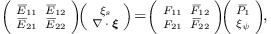
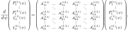
Equations (130) and (133), which involves only surface derivative operators, can be put in the following matrix form:
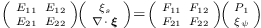 |
(134) |
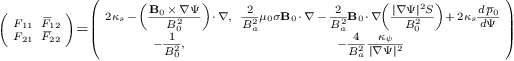
with the matrix elements given by
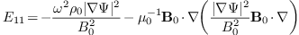 |
(135) |
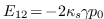 |
(136) |
 |
(137) |
 |
(138) |
 |
(139) |
 |
(140) |
 |
(141) |
 |
(142) |
Equations (134)-(142) agree with equations (25), (28), and (29) of Ref [3].
Using Eq. (129) to eliminate in Eq.
(127), we obtain

The equation for the divergence of [Eq. (95)] is written
 |
(144) |
Equations (143) and (144) can be put in the following matrix form
 |
(145) |
with the matrix elements given by
 |
(146) |
 |
(147) |
 |
(148) |
 |
(149) |
 |
(150) |
 |
(151) |
 |
(152) |
 |
(153) |
Equations (146)-(153) agree with Equations (26) and (27) in Ref.[3]. (It took me several months to manage to put the equations in the matrix form given here.)
Denote the strength of the equilibrium magnetic field at the magnetic
axis by  , the mass density at the magnetic axis
by
, the mass density at the magnetic axis
by  , and the major radius of the magnetic axis by
 . Define a characteristic speed
  ,
which is the Alfvén speed at the magnetic axis. Using the
Alfvén speed, we define a characteristic frequency
,
which is the Alfvén speed at the magnetic axis. Using the
Alfvén speed, we define a characteristic frequency  . Multiplying the matrix equation (134) by
 gives
gives
 |
(154) |
with new quantities defined as follows:  ,
,  ,
,  ,
,  ,
,
 ,
,  , and
, and  .
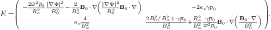
Using the equations (135), (136), (140),
(137), (138), and (142), the
expression of
.
Using the equations (135), (136), (140),
(137), (138), and (142), the
expression of  ,
, ,
,  ,
,  ,
, , and are written respectively as
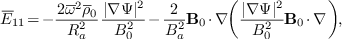 |
(155) |
 |
(156) |
 |
(157) |
 |
(158) |
 |
(159) |
 |
(160) |
where  ,
,  ,
,  .
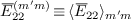
Next, consider re-normalizing the matrix equation (145).
Multiply the first equation of matrix equation (145) by
, giving
.
Next, consider re-normalizing the matrix equation (145).
Multiply the first equation of matrix equation (145) by
, giving
 |
(161) |
with the new matrix elements defined as follows:  ,
,
 , and
, and  . (Note that,
although the second equation of matrix equation (161) uses
. (Note that,
although the second equation of matrix equation (161) uses
 , instead of , as a
variable , it is actually identical with the second equation of matrix
equation (145) because the term is
multiplied by zero.) Using Eqs. (147), (148)
(149) , we obtain
, instead of , as a
variable , it is actually identical with the second equation of matrix
equation (145) because the term is
multiplied by zero.) Using Eqs. (147), (148)
(149) , we obtain
 |
(162) |
 |
(163) |
 |
(164) |
Note that, after the normalization, all the coefficients of the
resulting equations are of the order  , thus, are
suitable for accurate numerical calculation. Also note that, for typical
tokamak plasmas, the normalization factor is of
the order
, thus, are
suitable for accurate numerical calculation. Also note that, for typical
tokamak plasmas, the normalization factor is of
the order  , which is six order away from . Therefore the normalization performed here is
necessary for accurate numerical calculation. [If the normalizing factor
is two (or less) order from , then, from my
experience, it is usually not necessary to perform additional
normalization for the purpose of optimizing the numerical accuracy,
i.e., the original units system has provided a reasonable normalization.
Of course, suitable re-normalization will be of benefit to developing a
clear physical insight into the problem in question.]
, which is six order away from . Therefore the normalization performed here is
necessary for accurate numerical calculation. [If the normalizing factor
is two (or less) order from , then, from my
experience, it is usually not necessary to perform additional
normalization for the purpose of optimizing the numerical accuracy,
i.e., the original units system has provided a reasonable normalization.
Of course, suitable re-normalization will be of benefit to developing a
clear physical insight into the problem in question.]
In the above, we do not specify which coordinate system to use. In this
article, we will use the straight-line magnetic surface coordinate
system (i.e. flux coordinate system)  . The
details of this coordinate system are given in my notes on tokamak
equilibrium
(/home/yj/theory/tokamak_equilibrium/tokamak_equilibrium.tm).
. The
details of this coordinate system are given in my notes on tokamak
equilibrium
(/home/yj/theory/tokamak_equilibrium/tokamak_equilibrium.tm).
Any axisymetrical magnetic field consistent with the equilibrium
equation 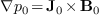 can be written in the form

where  . In the straight-line magnetic surface
coordinates system , the contra-variant form of
the equilibrium magnetic field is expressed as
. In the straight-line magnetic surface
coordinates system , the contra-variant form of
the equilibrium magnetic field is expressed as
 |
(165) |
where  . The covariant form of the equilibrium
magnetic field is given by
. The covariant form of the equilibrium
magnetic field is given by
 |
(166) |
where  is the Jacobian of
coordinate system.
is the Jacobian of
coordinate system.
The form of the radial differential operator  in
coordinates is given by
in
coordinates is given by
 |
(167) |
(Refer to my notes “tokamak_equilibrium.tm” for the proof.)
The MHD eigenmode equations (154) and (161)
involve two surface operators,  and
and 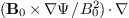 (they are called surface operators because they involve
only differential on magnetic surfaces). Next, we provide the form of
the two operators in flux coordinate system .
Using Eq. (165), the operator
(usually called magnetic differential operator) is written
(they are called surface operators because they involve
only differential on magnetic surfaces). Next, we provide the form of
the two operators in flux coordinate system .
Using Eq. (165), the operator
(usually called magnetic differential operator) is written
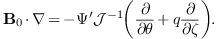 |
(168) |
Using the covariant form of the equilibrium magnetic field [Eq. (166)], the operator is written
 |
(169) |
 and
and 
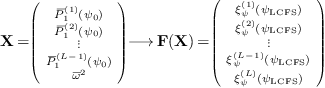
A perturbation  must be a periodic function of
the poloidal angle and toroidal angle , and thus can be expanded as the following two-dimensional
Fourier series,
must be a periodic function of
the poloidal angle and toroidal angle , and thus can be expanded as the following two-dimensional
Fourier series,
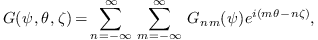 |
(170) |
where the expansion coefficient  is given by
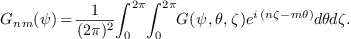 |
(171) |
Our next task is to derive the equations for the coefficients .
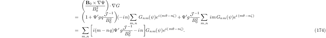
Next, consider the calculation of the surface operators acting on the above perturbation. Using Eqs. (168) and (170), we obtain

where  is a known function that is independent of
. Similarly, we have
is a known function that is independent of
. Similarly, we have
Using Eq. (169), we obtain
 ,
,  ,
,  , and
, and 
The elements of matrix , ,
, and are two dimensional
differential operators about  , which can be
called surface differential operators. As discussed above, we use
Fourier expansion to treat the differential with respect to and . In this method, we need to
take inner product between different Fourier harmonics (this is the
standard spectrum method, instead of the pseudo-spectral method). Noting
this, we recognize that it is useful to define the following inner
product operator:
, which can be
called surface differential operators. As discussed above, we use
Fourier expansion to treat the differential with respect to and . In this method, we need to
take inner product between different Fourier harmonics (this is the
standard spectrum method, instead of the pseudo-spectral method). Noting
this, we recognize that it is useful to define the following inner
product operator:

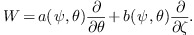
where  is a surface differential operator of the
following form
is a surface differential operator of the
following form
 |
(175) |
Because both of the coefficients in expression (175) are
independent of , it is ready to see that, for
 ,
, 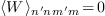 . This indicates that
with different
. This indicates that
with different  are
decoupled with each other.
are
decoupled with each other.
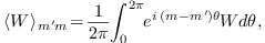
For notation ease,  is denoted by
  when
when  , i.e.,

[For the special case that is an algebra
operator  , equation (175) can be
reduced to
, equation (175) can be
reduced to
 |
(176) |
where  is independent of
because, as we will see below, is determined by
equilibrium quantities (for example,
is independent of
because, as we will see below, is determined by
equilibrium quantities (for example, 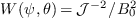 ), which is
axisymetrical. Expression (176) is a Fourier integration
over the interval
), which is
axisymetrical. Expression (176) is a Fourier integration
over the interval  , which can be efficiently
calculated by using the FFT algorithm (details are given in Chapter 13.9
of Ref. [5]).] After using the Fourier harmonics expansion
and taking the inner product, every element of the matrices
, which can be efficiently
calculated by using the FFT algorithm (details are given in Chapter 13.9
of Ref. [5]).] After using the Fourier harmonics expansion
and taking the inner product, every element of the matrices  , and becomes a
  matrix, where
  is the total number of the Fourier
harmonics included in the expansion. Taking the matrix
is the total number of the Fourier
harmonics included in the expansion. Taking the matrix  as an example, it is discretized as
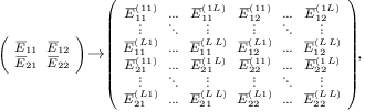 |
(177) |
where 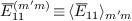 ,
, 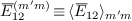 ,
,  ,
,
 . Next, let us derive the expressions of
  ,
,  ,
,  ,
,
 . The goal of the derivation is to perform the
surface differential operators so that all the inner products take the
form of the Fourier integration given by Eq. (176). For the
convenience of reference, the expression of matrix
is repeated here:
. The goal of the derivation is to perform the
surface differential operators so that all the inner products take the
form of the Fourier integration given by Eq. (176). For the
convenience of reference, the expression of matrix
is repeated here:
Then is written as

Making use of Eq. (173), equation (178) is written as
 |
(179) |
Note that all the operators within the inner operator  of the above equation are algebra operators. Therefore the calculation
of the inner product reduces to the calculation
of the Fourier integration (176), which can be efficiently
calculated by using the FFT algorithm (it is thus implemented in GTAW
code). Similarly, the discrete form of the other matrix elements are
written respectively as:
of the above equation are algebra operators. Therefore the calculation
of the inner product reduces to the calculation
of the Fourier integration (176), which can be efficiently
calculated by using the FFT algorithm (it is thus implemented in GTAW
code). Similarly, the discrete form of the other matrix elements are
written respectively as:


Next, consider the discrete form of the normalized
matrix, which is given by
 |
(183) |
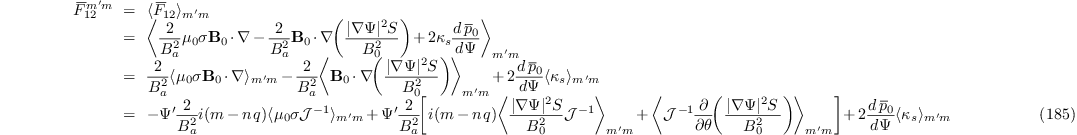
Using Eqs. (139) and (159), we obtain

 |
(186) |
 |
(187) |
Next, we derive the discrete form of matrix and
. Before doing this, we examine matrix equation
(161), which can be written as
 |
(188) |
Using the expression of the operator , i.e.,
 |
(189) |
equation (188) is written as
 |
(190) |
Define the first matrix on the r.h.s of the above equation as  , then
  , and
, and  and
and  are given by
 |
(191) |
Then
 |
(192) |
 |
(193) |

 |
(194) |
The formula for calculating the right-hand side of Eq. (194) is given in Sec. 8.6.

 |
(196) |


In the GTAW code, the weight functions appearing in the Fourier integration are numbered as follows:
 |
(199) |
 |
(200) |
 |
(201) |
 |
(202) |
 |
(203) |
 |
(204) |
 |
(205) |
 |
(206) |
 |
(207) |
 |
(208) |
 |
(209) |
 |
(210) |
 |
(211) |
The formulas for calculating the equilibrium quantities, such as the
geodesic curvature  , normal curvature
  , and the local magnetic shear
  , are
given in Sec. 8.4.
, are
given in Sec. 8.4.
In the GTAW code, the matrix elements  and
and  are multiplied by
  (check
whether this will make
(check
whether this will make  a root of
  ?). After this, the matrix elements
can be written in the following form
?). After this, the matrix elements
can be written in the following form
 |
(212) |
where  and
and  are
are  matrix which are both independent of
  .
.
The continua are determined by the condition that ,
which is the condition that the matrix equation  has nonzero solutions. Using Eq. (212), the matrix equation
can be written
has nonzero solutions. Using Eq. (212), the matrix equation
can be written
 |
(213) |
Thus finding that can make
have nonzero solution reduces to finding the eigenvalues of the
generalized eigenvalue problem in Eq. (213). In GTAW code,
the generalized eigenvalue problem in Eq. (213) is solved
numerically by using the zggev subroutine in Lapack
library. The numerical results of the continuous spectrum are given in
Sec. 8.2.
Before we give the numerical solution for the continuous spectrum, we consider some approximations that can be made when solving continuous spectrum.
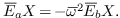
Examining the expression (138) for matrix element  , we find that the first term of
can be written as
, we find that the first term of
can be written as
 |
(214) |
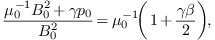
where 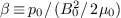 , while the second term of
can be written as
, while the second term of
can be written as
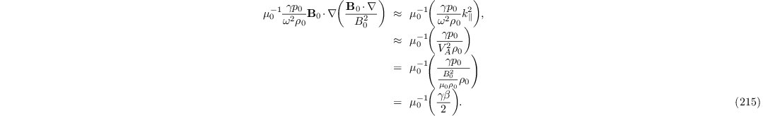
where  is the parallel wave vector and we have
used the approximation
is the parallel wave vector and we have
used the approximation  . Using Eqs. (214)
and (215), the ratio of the second term to the first term
of is written as
. Using Eqs. (214)
and (215), the ratio of the second term to the first term
of is written as  . For
low
. For
low  (
( ) equilibrium, the
ratio is small and therefore the second term of
can be dropped. This approximation is called the slow sound
approximation in the literature[6, 7].
Numerical results indicate this approximation will remove all the sound
continua while keeping the Alfven continua nearly unchanged.
) equilibrium, the
ratio is small and therefore the second term of
can be dropped. This approximation is called the slow sound
approximation in the literature[6, 7].
Numerical results indicate this approximation will remove all the sound
continua while keeping the Alfven continua nearly unchanged.
If we set all the thermal pressure terms in  and
to be zero (this is equivalent with setting
and
to be zero (this is equivalent with setting  ), the sound wave will be removed from the system.
This approximation is called zero beta limit in literature[6].
Numerical results indicate the zero beta limit will remove all the sound
continua. Compared with the slow sound approximation, the zero beta
limit will make the frequency of the Alfven continua a little lower, and
make the zeroth continua gaps (BAE gaps) disappear[7].
), the sound wave will be removed from the system.
This approximation is called zero beta limit in literature[6].
Numerical results indicate the zero beta limit will remove all the sound
continua. Compared with the slow sound approximation, the zero beta
limit will make the frequency of the Alfven continua a little lower, and
make the zeroth continua gaps (BAE gaps) disappear[7].
Consider the form of matrix in the cylindrical
geometry limit, in which the equilibrium quantities are independent of
poloidal angle. Equation (284) indicates that the geodesic
curvature is zero in this case. Thus, the matrix
elements and  are zero.
Next, consider the matrix elements
are zero.
Next, consider the matrix elements  and . Because all equilibrium quantities are independent of the
poloidal angle, different poloidal harmonics of the perturbation are
decoupled. Therefore, we can consider a perturbation with a single
poloidal mode number . For a poloidal harmonic with poloidal mode number
and . Because all equilibrium quantities are independent of the
poloidal angle, different poloidal harmonics of the perturbation are
decoupled. Therefore, we can consider a perturbation with a single
poloidal mode number . For a poloidal harmonic with poloidal mode number
 , matrix element is
written
, matrix element is
written

and matrix element is written

The continua are the roots of the equation  ,
which, in the cylindrical geometry limit, reduces to
,
which, in the cylindrical geometry limit, reduces to
 |
(218) |
Two branches of the roots of Eq. (218) are given by  and
and  , respectively. The
equation is written
, respectively. The
equation is written
 |
(219) |
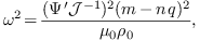
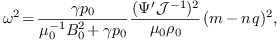
which gives
 |
(220) |
which is the Alfvén branch of the continua. Figure 1a
plots the results of Eq. (220). The equation is written
 |
(221) |
which is the sound branch of the continua. Figure 1b plots the results of Eq. (221).
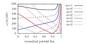 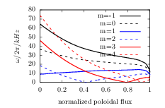 |
Figure 1. |
Figures 2 compares the Alfven continua in the cylindrical limit with those in the toroidal geometry. The results indicate that the Alfven continua in the toroidal geometry reconnect, forming gaps near the locations where the Alfven continua in the cylindrical limit intersect each other.
The result in Eq. (220) is not clear from the physical point of view since it involves the Jacobian, which is a mathematical factor due to the freedom in the choice of coordinates. Next, we try to write the right-hand side of Eq. (220) in more physical form. In cylindrical geometry limit, magnetic surfaces are circular. Thus the radial coordinate can be chosen to be the geometrical radius of the circular magnetic surface, and the usual poloidal angle (i.e., equal-arc angle) can be used as the poloidal coordinate. Then the poloidal magnetic flux is written as
 |
(222) |
where  is the length of the cylinder. We know
that used in the Grad-Shafranov equation is
related to
is the length of the cylinder. We know
that used in the Grad-Shafranov equation is
related to  by
by
 |
(223) |
Using Eqs. (222) and (223), we obtain
 |
(224) |
Next, we calculate the Jacobian , which is
defined by
 |
(225) |
Since we choose  and
and  (the
positive direction of is count clockwise when
observers view along the positive direction of
(the
positive direction of is count clockwise when
observers view along the positive direction of  ),
the above equation is written
),
the above equation is written

Using Eqs. (224) and (226) ,  is written
 |
(227) |
Using these, Eq. (220) is written
 |
(228) |
Using the definition of safety factor in the cylindrical geometry
 |
(229) |
equation (228) is written
 |
(230) |
In the cylindrical geometry, the parallel (to equilibrium magnetic field) wave-number is given by
 |
(231) |
Using this, Eq. (230) is written
 |
(232) |
Using the definition of Alfven speed  , the above
equation is written as
, the above
equation is written as
 |
(233) |
which gives the well known Alfven resonance condition. For later use, define
 |
(234) |
then Eq. (228) is written as  .
.
Similarly, by using Eq. (227), equation (217)
for is written as
Then equation reduces to
 |
(235) |
 |
(236) |
where  ,
,  . Equation (166) gives the sound branch of the continua. For present
tokamak plasma parameters,
. Equation (166) gives the sound branch of the continua. For present
tokamak plasma parameters,  is usually one order
smaller than
is usually one order
smaller than  . Thus, equation (236)
indicates the sound continua are much smaller than the Alfven continua
for the same and .
. Thus, equation (236)
indicates the sound continua are much smaller than the Alfven continua
for the same and .
In the cylindrical geometry, continua with different poloidal mode
numbers will intersect each other, as shown in Fig. 1.
Next, we calculate the radial location of the intersecting point of two
continua with poloidal mode number and  , respectively. In the intersecting point, we have
 |
(237) |
i.e.
 |
(238) |
which gives
 |
(239) |
or
 |
(240) |
Inspecting the expression for in Eq. (323),
i.e.,

we know that only the case in Eq. (240) is possible, which gives
 |
(241) |
which further reduces to
 |
(242) |
The above equation determines the radial location where the continuum intersect the continuum.
Note that a mode with two poloidal modes has two corresponding resonant
surfaces. For the case where the mode has and
poloidal harmonics, the resonant surfaces are
respectively  and
and  . Note
that the value of
. Note
that the value of  given in Eq. (242)
is between the above two values.
given in Eq. (242)
is between the above two values.
In toroidal geometry, the different poloidal modes are coupled, and the continuum will “reconnect” to form a gap in the vicinity of the original intersecting point, as shown in Fig. 2. Therefore the original intersecting point, Eq. (242), gives the approximate location of the gap. Furthermore, using Eq. (242), we can determine the frequency of the intersecting point, which is given by
 |
(243) |
which can be further written
 |
(244) |
According to the same reasoning given in the above, Eq. (244) is an approximation to the center frequency of the TAE gap. The frequency and the location given above are also an approximation to the frequency and location of the TAE modes that lie in the gap.
For the ellipticity-induced gap (EAE gap), which is formed due to the
coupling of and  harmonics, the location is approximately determined by
 |
(245) |
which gives
 |
(246) |
and the approximate center angular frequency is
 |
(247) |
which can be written as
Generally, for the gap formed due to the coupling of
and  harmonics, we have
which gives
 |
(248) |
and
 |
(249) |
Equation (249) can also be written as
 |
(250) |
After using Fourier spectrum expansion and taking the inner product over
, Eq. (190) can be written as the
following system of ordinary differential equations:
 |
(251) |
where is the total number of the poloidal
harmonics included in the Fourier expansion, the matrix elements  are functions of
  and . Next, we specify the boundary condition for the
system. Note that equations system (251) has
and . Next, we specify the boundary condition for the
system. Note that equations system (251) has  first-order differential equations, for which we need to
specify boundary conditions to make the solution
unique. The geometry determines that the radial displacement at the
magnetic axis must be zero, i.e.,
first-order differential equations, for which we need to
specify boundary conditions to make the solution
unique. The geometry determines that the radial displacement at the
magnetic axis must be zero, i.e.,
 |
(252) |
We consider only the modes that vanish at the plasma boundary, for which we have the following boundary conditions:
 |
(253) |
Now Eqs. (252) and (253) provide boundary conditions, half of which are at the boundary
 and half are at the boundary
  .
Therefore equations system (251) along with the boundary
conditions Eqs. (252) and (253) constitutes a
standard two-points boundary problem[5]. Note, however,
that we are solving a eigenvalue problem, for which there is an
additional equation for :
.
Therefore equations system (251) along with the boundary
conditions Eqs. (252) and (253) constitutes a
standard two-points boundary problem[5]. Note, however,
that we are solving a eigenvalue problem, for which there is an
additional equation for :
 |
(254) |
This increases the number of equations by one and so we need one
additional boundary condition. Note that, by eliminating all  , equations system (251) can be written as a
system of second-order differential equations for
, equations system (251) can be written as a
system of second-order differential equations for  .
Further note that the unknown functions satisfy
homogeneous equations and homogeneous boundary conditions, which
indicates that if with
.
Further note that the unknown functions satisfy
homogeneous equations and homogeneous boundary conditions, which
indicates that if with  are solutions, then
  are also solutions to the
original equations, where
are also solutions to the
original equations, where  is a constant.
Therefore the value of the derivative of
is a constant.
Therefore the value of the derivative of  at the
boundary have one degree of freedom. Due to this fact, one of the
derivatives
at the
boundary have one degree of freedom. Due to this fact, one of the
derivatives  ,
,  ,…,
,…,
 at
at  can be set to be a
nonzero value. For example, setting the value of
at to be
can be set to be a
nonzero value. For example, setting the value of
at to be  and making use
of
and making use
of  at , we obtain
 |
(255) |
which can be solved to give
 |
(256) |
which provides the additional boundary condition we need. In the present
version of my code, for convenience, I directly set the value of  to a small value, instead of using Eq. (256).
The following sketch map describes the function
to a small value, instead of using Eq. (256).
The following sketch map describes the function  for which we need to find roots in the shooting process.
 |
(257) |
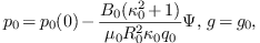
To benchmark GTAW code, we use it to calculate the continua and gap modes of the Solovev equilibrium and compare the results with those given by NOVA code. The Solovev equilibrium used in the benchmark case is given by
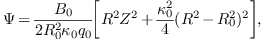 |
(258) |
 |
(259) |
with  ,
,  ,
,  ,
,
 , and
, and  . The flux surface
with the minor radius being
. The flux surface
with the minor radius being  (corresponding to
 ) is chosen as the boundary flux surface. Main
plasma is taken to be Deuterium and the number density is taken to be
uniform with
) is chosen as the boundary flux surface. Main
plasma is taken to be Deuterium and the number density is taken to be
uniform with  . Figure 3 compares the
Alfven continua calculated by NOVA and GTAW, which shows good agreement
between them.
. Figure 3 compares the
Alfven continua calculated by NOVA and GTAW, which shows good agreement
between them.
|
Figure 3. Comparison of the |
A gap mode with frequency  is found in the NAE
gap by both NOVA and GTAW. The poloidal mode numbers of the two dominant
harmonics are
is found in the NAE
gap by both NOVA and GTAW. The poloidal mode numbers of the two dominant
harmonics are  and
and  , which
is consistent with the fact that a NAE is formed due to the coupling
between and
, which
is consistent with the fact that a NAE is formed due to the coupling
between and  harmonics.
Before comparing the radial structure of the poloidal harmonics given by
the two codes, a discussion about the assumption adopted in NOVA is
desirable. As is pointed out by Dr. Gorelenkov, NOVA at present is
restricted to up-down symmetric equilibrium and, for this case, it can
be shown that the amplitude of all the radial displacement can be
transformed to real numbers. For this reason, NOVA use directly real
numbers for the radial displacement in its calculation. In GTAW code,
the amplitude of the poloidal harmonics of the radial displacement are
complex numbers. The Solovev equilibrium used here is up-down symmetric
and the results given by GTAW indicate the poloidal harmonics of the
radial displacement can be transformed (by multiplying a constant such
as
harmonics.
Before comparing the radial structure of the poloidal harmonics given by
the two codes, a discussion about the assumption adopted in NOVA is
desirable. As is pointed out by Dr. Gorelenkov, NOVA at present is
restricted to up-down symmetric equilibrium and, for this case, it can
be shown that the amplitude of all the radial displacement can be
transformed to real numbers. For this reason, NOVA use directly real
numbers for the radial displacement in its calculation. In GTAW code,
the amplitude of the poloidal harmonics of the radial displacement are
complex numbers. The Solovev equilibrium used here is up-down symmetric
and the results given by GTAW indicate the poloidal harmonics of the
radial displacement can be transformed (by multiplying a constant such
as  ) to real numbers. After transforming the
radial displacement to real numbers, the results can be compared with
those of NOVA. Figure 4 compares the radial structure of
the dominant poloidal harmonics
) to real numbers. After transforming the
radial displacement to real numbers, the results can be compared with
those of NOVA. Figure 4 compares the radial structure of
the dominant poloidal harmonics  given by the two
codes, which indicates the results given by the two codes agree with
each other well.
given by the two
codes, which indicates the results given by the two codes agree with
each other well.
|
Figure 4. The dominant poloidal
harmonics ( |
|
Figure 5. Slow sound approximation of the |
Figure 6 plots the mode structure of the NAE on  plane, which shows that the mode has an anti-ballooning
structure, i.e., the mode is stronger at the high-field side than at the
low-field side.
plane, which shows that the mode has an anti-ballooning
structure, i.e., the mode is stronger at the high-field side than at the
low-field side.
|
Figure 6. Two dimension mode
structure of the NAE in Fig. 4. The dashed line in
the figure indicates the boundary magnetic surface and the small
circle indicates the inner boundary used in the numerical
calculation.
|
|
Figure 7. Real part (a), imaginary part (b), and
absolute value of the amplitude (c) of the poloidal harmonics of a
|
|
Figure 8. Slow sound approximation of the
continua of the Solovev equilibrium. Also plotted are the
frequency of the TAE ( |
For the case that  , a TAE with
  is found in the TAE gap. The radial dependence of the poloidal harmonics
of the mode is plotted in Fig. 9. Figure 10
plots the frequency of the mode on the Alfven continua graphic.
is found in the TAE gap. The radial dependence of the poloidal harmonics
of the mode is plotted in Fig. 9. Figure 10
plots the frequency of the mode on the Alfven continua graphic.
|
Figure 9. Real part (a), imaginary
part (b), and absolute value of the amplitude (c) of the poloidal
harmonics of a |
|
Figure 10. Slow sound approximation
of the continua of the Solovev equilibrium. Also plotted are the
frequency of the TAE ( |
The content in this section has been published in my 2014 paper[8].
The tokamak equilibrium used in this paper is reconstructed by EFIT code
by using the information of profiles measured in EAST experiment[9]. The shape of flux surfaces within the last-closed-flux
surface (LCFS) are plotted in Fig. 11, where  curves are also plotted. In the paper, I said that the
equilibrium was a double-null configuration with the LCFS connected to
the lower X point. This is wrong. The configuration with the LCFS
connected to the lower X point should be called lower single null
configuration. The double-null configuration is a configuration with
LCFS connected to both the lower and upper X points. In practice, if the
spacial seperation between the flux surface connected to the low X point
and the flux surface connected to the upper X point,
curves are also plotted. In the paper, I said that the
equilibrium was a double-null configuration with the LCFS connected to
the lower X point. This is wrong. The configuration with the LCFS
connected to the lower X point should be called lower single null
configuration. The double-null configuration is a configuration with
LCFS connected to both the lower and upper X points. In practice, if the
spacial seperation between the flux surface connected to the low X point
and the flux surface connected to the upper X point,  ,
is smaller than a value (e.g. 1cm), the configuration can be considered
as a double null configuration, where is the
spacial separation between the two flux surfaces on the low-field side
of the midplane.
,
is smaller than a value (e.g. 1cm), the configuration can be considered
as a double null configuration, where is the
spacial separation between the two flux surfaces on the low-field side
of the midplane.
The profiles of safety factor, pressure, and electron number density are plotted in Fig. 12.
The mass density is calculated from  , where
  is the mass of the main
ions (deuterium ions in this discharge),
is the mass of the main
ions (deuterium ions in this discharge),  is the
number density of the ions, which is inferred from
is the
number density of the ions, which is inferred from  by using the neutral condition
  (impurity ions
are neglected).
(impurity ions
are neglected).
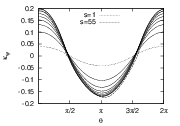 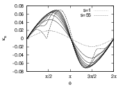 |
Figure 13. Normal and geodesic magnetic
curvature as a function of the poloidal angle. Different lines in
the figure correspond to different magnetic surfaces.
|
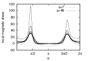 |
Figure 14. Negative local magnetic
shear |
 |
Figure 15. |
The eigenfrequency of Eq. (213), ,
as a function of the radial coordinate gives the continua for the
equilibrium. It can be proved analytically that the eigenfrequency of
Eq. (213), , is a real number (I do
not prove this). Making use of this fact, we know that a crude method of
finding the eigenvalue of Eq. (213) is to find the zero
points of the real part of the determinant of .
Since, in this case, both the independent variables and the value of the
function are real, the zero points can be found by using a simple
one-dimension root finder. This method was adopted in the older version
of GTAW (bisection method is used to find roots). In the latest version
of GTAW, as mentioned above, the generalized eigenvalue problem in Eq.
(213) is solved numerically by using the
zggev subroutine in Lapack library. (The eigenvalue
problem is solved without the assumption that is
real number. The eigenvalue obtained from the
routine is very close to a real number, which is consistent with the
analytical conclusion that the eigenvalue must
be a real number.)
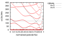
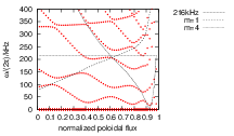
Figure 16 plots the eigenfrequency of Eq. (213)
as a function of the radial coordinate  . The
result is calculated in the slow sound approximation, thus giving only
the Alfven branch of the continua. Also plotted in Fig. 16
are the Alfven continua in the cylindrical limit. As shown in Fig. 16, the Alfven continua in toroidal geometry do not intersect
each other, thus forming gaps at the locations where the cylindrical
Alfven continua intersect each other.
. The
result is calculated in the slow sound approximation, thus giving only
the Alfven branch of the continua. Also plotted in Fig. 16
are the Alfven continua in the cylindrical limit. As shown in Fig. 16, the Alfven continua in toroidal geometry do not intersect
each other, thus forming gaps at the locations where the cylindrical
Alfven continua intersect each other.
The first gap, which is formed due to the coupling of sound wave and
Alfven wave, starts from zero frequency. This gap is called BAE gap
since beta-induced Alfven eigenmode (BAE) can exist in this gap. The
second gap is called TAE gap, which is formed mainly due to the coupling
of and poloidal
harmonics. The third gap is called EAE gap, which is formed mainly due
to the coupling of and
poloidal harmonics. The fourth gap is called NAE gap, which is formed
due to the coupling of and
poloidal harmonics. A gap can be further divided into sub-gaps according
to the two dominant poloidal harmonics that are involved in forming the
gap. For example, a sub-gap of the TAE gap is the one that is formed
mainly due to the coupling of  and harmonics. For the ease of discussion, we call this
sub-gap “
and harmonics. For the ease of discussion, we call this
sub-gap “ sub-gap”, where the two
numbers stand for the poloidal mode numbers. The frequency range of a
sub-gap is defined by the frequency difference of the two extreme points
on the continua. The radial range of the sub-gap can be defined as the
radial region whose center is the location of one of the extreme points
on the continua, width is the half width between the neighbor left and
right extreme points.
sub-gap”, where the two
numbers stand for the poloidal mode numbers. The frequency range of a
sub-gap is defined by the frequency difference of the two extreme points
on the continua. The radial range of the sub-gap can be defined as the
radial region whose center is the location of one of the extreme points
on the continua, width is the half width between the neighbor left and
right extreme points.
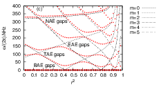 |
Figure 16. |
Figure 17 compares the continua of the full ideal MHD model
with those of slow sound and zero
approximations. The results indicate that the slow sound approximation
eliminates the sound continua while keeps the Alfven continua almost
unchanged. The zero approximation eliminates the
BAE gap.
(Numerical results indicate that the eigenvalue
is always grater than or equal to zero. Can this point be proved
analytically?)
In order to verify the numerical convergence about the number of the
poloidal harmonics included in the expansion, we compares the results
obtained when the poloidal harmonic numbers are truncated in the range
 and those obtained when the truncation region is
 . The results are plotted in Fig. 18,
which shows that the two results agree with each other very well for the
low order continua in the core region of the plasma. For continua in the
edge region or higher order continua, there are some discrepancies
between the two results. These discrepancies are due to that higher
order poloidal harmonics are needed in evaluating the continua for those
cases.
. The results are plotted in Fig. 18,
which shows that the two results agree with each other very well for the
low order continua in the core region of the plasma. For continua in the
edge region or higher order continua, there are some discrepancies
between the two results. These discrepancies are due to that higher
order poloidal harmonics are needed in evaluating the continua for those
cases.
The  Alfven continua are plotted in Fig. 19,
which shows that there are more TAE gaps than those of the
Alfven continua are plotted in Fig. 19,
which shows that there are more TAE gaps than those of the  case. The number of gaps is roughly given by
  for a monotonic profile[10].
Remarks: If, instead of the definition (169), we define the
operator as
 |
(260) |
then, can we still obtain correct results for the continuous spectrum?
When I began to work on the calculation of the continuous spectrum, I
noticed that the definition (169), instead of (260),
is adopted in Cheng's paper[3]. By intuition, I thought the
definition (260) should work as well as (169).
Since the definition (260) is simpler than (169)
(there is no additional minus in (260)), I prefer using the
definition (260). This choice does not cause me trouble
when I use symmetrical truncation of the poloidal harmonics. Trouble
appears when I try using asymmetrical truncation of the poloidal
harmonics. For example, when asymmetrical truncation of the poloidal
harmonics is used (e.g. poloidal harmonics in the range  ),
it is easy to verify analytically that the determinant of the resulting
matrix for the case is zero for any values of
. It is obvious that this will not give correct
results for the continuous spectrum. It took me two days to find out the
definition in (169) must be used in order to deal with
asymmetrical truncation of poloidal harmonics. In summary, the advantage
of using the definition (169) over (260), is
that the former can deal with the asymmetrical truncation of the
poloidal harmonics, while the latter is limited to the case of
symmetrical truncation.
),
it is easy to verify analytically that the determinant of the resulting
matrix for the case is zero for any values of
. It is obvious that this will not give correct
results for the continuous spectrum. It took me two days to find out the
definition in (169) must be used in order to deal with
asymmetrical truncation of poloidal harmonics. In summary, the advantage
of using the definition (169) over (260), is
that the former can deal with the asymmetrical truncation of the
poloidal harmonics, while the latter is limited to the case of
symmetrical truncation.
When analyzing the modes calculated numerically, we need to distinguish two kinds of modes: the continuum modes and the gap modes. In principle, the continuum mode is defined as the mode whose frequency is within the Alfven continua while the gap mode is defined as the mode whose frequency is within the frequency gap of the Alfven continua. However, for realistic equilibria, any given frequency will touch the continua at one of the radial locations.
However, for realistic structure of continua, both the range and the
center of the frequency of a gap change with the radial coordinate, as
is shown in Fig. 16. As a result, a given frequency usually
can not be within a gap for all radial locations, i.e., the frequency
usually intersects the Alfven continua at some radial locations. These
locations are the Alfven resonant surfaces. As is pointed out in Ref.
[?], the mode structure have singularity given by  at the resonant surface, where
  is
the radial coordinate of the resonant surface and
is
the radial coordinate of the resonant surface and  can have finite discontinuity.
In practice, continuum modes can be easily distinguished from gap modes by examining the radial structure of the poloidal harmonics of the mode. If the radial mode structure has dominant singularities at the Alfven resonant surfaces, then the modes are continua modes. If the dominant peaks of the mode are not at the Alfven resonant surfaces, then the mode is probably a gap mode (further confirmation can be obtained by examining poloidal mode number of the dominant harmonics, discussed later). The mode structure of gap modes can also have singular peak at the resonant surface, but the peak is usually smaller than the dominant peak.
Mode structure of a TAE mode is plotted in Fig.
20
Fig. 22. plots the radial mode structure of another TAE
with frequency  .
.
An example of ellipticity-induced Alfven Eigenmode (EAE) is plotted in
Fig. 24. The mode is identified as an EAE mode because it
satisfies the following three requirements: (1) the mode has two
dominant harmonics with poloidal mode number differing by two ( and  for this case); (2) the
frequency of the mode
for this case); (2) the
frequency of the mode  is within in the continuum
gap formed due to the coupling of these two poloidal harmonics; (3) the
location of the peak of the radial mode structure is within the
continuum gap.
is within in the continuum
gap formed due to the coupling of these two poloidal harmonics; (3) the
location of the peak of the radial mode structure is within the
continuum gap.
 |
An example of non-circularity-induced Alfven Eigenmode (NAE) is plotted in Fig. 26.
 |
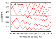 |
Figure 29. The frequency of the EAE mode given
in Fig. 28. (H)
|
In this section, we derive formulas for calculating the geodesic
curvature and normal curvature in magnetic surface coordinate system
 . The derivation looks tedious but the final
results are compact (especially for the geodesic curvature ). The magnetic curvature is defined by
. The derivation looks tedious but the final
results are compact (especially for the geodesic curvature ). The magnetic curvature is defined by  ,
which can be further written as
,
which can be further written as

In magnetic surface coordinate system , equation
(261) is written as
Using  , we obtain
  . Using
this, the three partial derivatives in the above equation are written
respectively as
. Using
this, the three partial derivatives in the above equation are written
respectively as

 |
(264) |
 |
(265) |
Using these,  is written as

The component is defined by  .
Using Eq. (262), is written as
.
Using Eq. (262), is written as
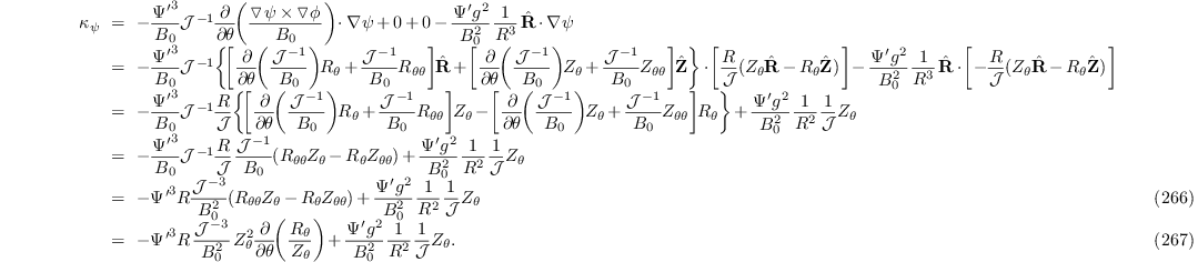
Equation (266) is used in GTAW code to calculate . Equation (267) is not suitable for numerical
calculation because  , which appears both in
numerator and denominator, can be very small, leading to significant
errors in the numerical results. [My notes: the bad results calculated
by Eq. (267) in my code reminded me that Eq. (266)
may be better. I switch back to adopt Eq. (266) and the
results clearly show that the results given by Eq. (266)
are indeed better than those of Eq. (267), as shown in Fig.
30.]
, which appears both in
numerator and denominator, can be very small, leading to significant
errors in the numerical results. [My notes: the bad results calculated
by Eq. (267) in my code reminded me that Eq. (266)
may be better. I switch back to adopt Eq. (266) and the
results clearly show that the results given by Eq. (266)
are indeed better than those of Eq. (267), as shown in Fig.
30.]
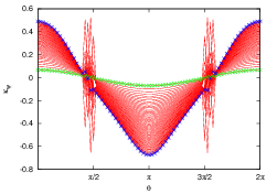 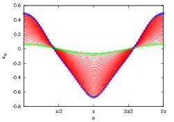 |
Figure 30. The normal curvature |
Next, consider the calculation of the surface component of , the geodesic curvature , which is
defined by
 |
(268) |
Using

and Eq. (263), we obtain


Using Eqs. (270), (271), and (272), equation (268) is written as

The terms in the first line of Eq. (273) is written as

Noting that
 |
(275) |
and
 |
(276) |
expression (274) is written as

The first two terms on the second line of Eq. (273) can be written as
 |
(278) |
The sum of the expression (278) and the first term of expression (277) is written as
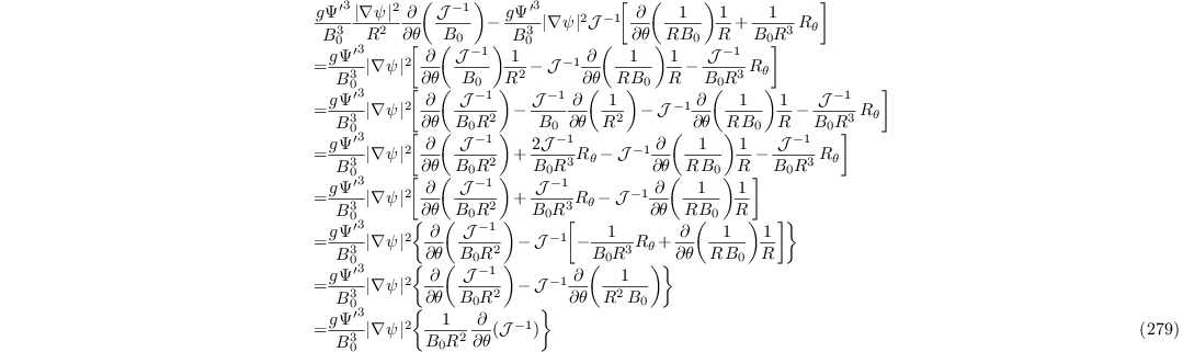
Using the above results, is written as
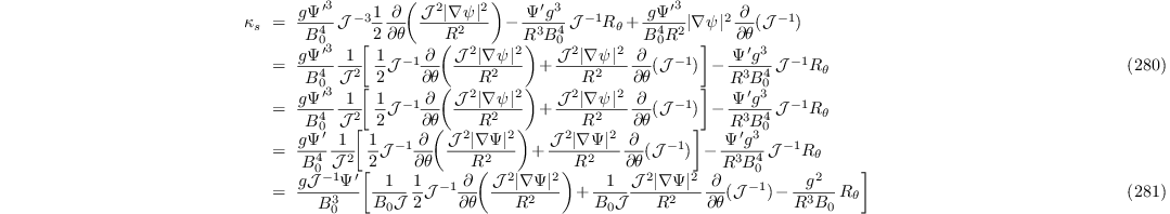
Using

equation (281) is written


Excluding the  term, the other terms on the r.h.s
of the above equation are written
term, the other terms on the r.h.s
of the above equation are written

Therefore equation (281) is written
 |
(282) |
which agrees with the formula given in Ref. [6]. Equation
(282) takes a very simple form, and provides a clear
physical meaning for the geodesic curvature: is
proportional to the poloidal derivative of the magnetic field strength.
Equation (284) indicates that the geodesic curvature is
zero for an equilibrium configuration that is uniform in poloidal
direction. Note that this formula for is valid
for arbitrary Jacobian. (Remarks: When I derived the formula of for the first time, I found that
can be written in the simple form given by Eq. (282) for
the equa-arc length Jacobian. Later I found that
can also be written in the simple form given by Eq. (282)
for the Boozer Jacobian. This makes me realize that the simple form
given by Eq. (282) may be universally valid for arbitrary
Jacobian. However, I did not verify this then. About two years later, I
reviewed this notes and succeeded in providing the derivation given
above. The derivation given above seems to be tedious and may be greatly
simplified in some aspects. But, at present, the above derivation is the
only one that I can provide.)
If we choose the equal-arc Jacobian, then Eq. (280) becomes relatively simple:
 |
(283) |
This form is implemented in GTAW code. Figure 31 gives the
results for calculated by using Eq. (283).
I have verified numerically that the results given by Eqs. (282)
and (283) agree with each other.
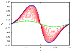 |
Figure 31. The geodesic magnetic
curvature |
The negative local magnetic shear is defined by
 |
(284) |
There are two ways of calculating . The first way
is to calculate in cylindrical coordinate
system; the second one is in flux coordinate system. Next, consider the
first way. We have

Using this, Eq. (284) is written as

Next, we work in cylindrical coordinates and obtain

and
 |
(288) |
Using Eq. (288), Eq. (286) is written as
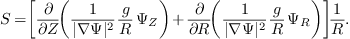 |
(289) |
The two partial derivatives appearing in the above equation can be calculated to give


Using these, we obtain
 |
(292) |
(The above results for has been verified by
using Mathematica Software.) The results calculated by using Eq. (292) are plotted in Fig. 32.
Next, we consider the calculation of in the flux
coordinates system . The
term can be written as

 |
(294) |
By using the curl formula in generalized coordinates ,
we obtain

Using Eqs. (294) and (295), the negative local magnetic shear [Eq. (284)] is written as
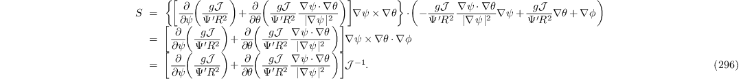
Note that the partial derivatives  and
and  in Eq. (296) is taken in the
coordinates and they are usually different from their counterparts in
coordinates. In Eq. (296), the
partial derivatives are operating on equilibrium quantity, which is
independent of and . In
this case, the partial derivatives in the two sets of coordinates are
equal to each other. Figure 33 plots the poloidal
dependence of local magnetic shear and
in Eq. (296) is taken in the
coordinates and they are usually different from their counterparts in
coordinates. In Eq. (296), the
partial derivatives are operating on equilibrium quantity, which is
independent of and . In
this case, the partial derivatives in the two sets of coordinates are
equal to each other. Figure 33 plots the poloidal
dependence of local magnetic shear and  .
.
Next, let us examine the flux surface average of ,
which is written as
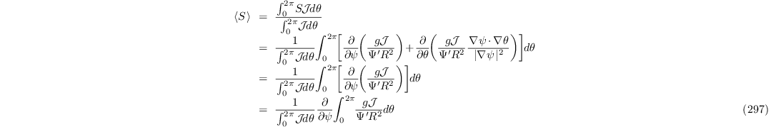
Note that the global safety factor is given by
 |
(298) |
Using this, equation (297) is written as
 |
(299) |
Equation (299) provides a way to verify the correctness of
the numerical implementation of . Figure 34
compares  with
with  , which
shows that the two results agree with each other well.
, which
shows that the two results agree with each other well.
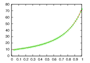 |
Figure 34. |

Next, consider the calculation of matrix elements .
In cylindrical coordinates, we have
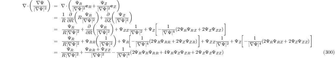
Using this, is written

Equation (301) is used in GTAW to calculate .
can also be calculated in the magnetic surface
coordinates.
 |
(302) |
the term on the r.h.s of the above equation is written as

The first term on the r.h.s of Eq. (303) is written as

The second term on the r.h.s of Eq. (303) is written as

Using these, Eq. (302) is finally written as

In experiments, the beam emission spectroscopy (BES) and microwave
reflectometer can measure electron density fluctuation. The electron
cyclotron emission (ECE) radiometer can measure electron temperature
fluctuation. In the ideal MHD theory, we assume that  ,
,
 , and the mass density is given approximately by
 . Then the linearized continuity equation,
  , is written as
 |
(307) |
which gives relationship between the density fluctuation and plasma
displacement. Similarly, in the ideal MHD theory, we assume that  ,
,  , and
, and  .
Then the linearized equation of state,
.
Then the linearized equation of state,  , is
written as
, is
written as
 |
(308) |
Using Eq. () to eliminate  , Eq. () is written as
 |
(309) |
 |
(310) |
 |
(311) |
The continuity equation is written as
 |
(312) |
Neglecting the compressible term, the above equation is written as
 |
(313) |
Using  and , the above
equation is written as
and , the above
equation is written as
 |
(314) |
Equation (314) relates the radial displacement obtained
from a eigenvalue code with the density perturbation  ,
which can be measured by the reflectometer in experiments.
,
which can be measured by the reflectometer in experiments.
We know that the radial plasma displacement is
related to the perturbed thermal pressure through the relation:
 |
(315) |
Neglecting the compressible term, the above equation is written as
 |
(316) |
and

Next, we derive the expression for the parallel and poloidal wave-number of a perturbation of the form
 |
(317) |
where are the flux coordinators, with and being the generalized poloidal
and toroidal angles. The parallel (to the local equilibrium magnetic
field) wave vector, , is defined by
 |
(318) |
where  is the phase angle change of the
perturbation when moving a distance of
is the phase angle change of the
perturbation when moving a distance of  along the
local equilibrium magnetic field. According to Eq. (317),
the phase change can be written as
along the
local equilibrium magnetic field. According to Eq. (317),
the phase change can be written as
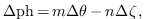 |
(319) |
where  and
and  are the change
in the toroidal and poloidal angles when we move a distance of along the magnetic field. Use Eq. (319), Eq.
(318) is written
are the change
in the toroidal and poloidal angles when we move a distance of along the magnetic field. Use Eq. (319), Eq.
(318) is written
 |
(320) |
Noting that the safety factor is given by
 |
(321) |
(which is exact since we are using flux coordinator, in which magnetic
field lines are straight on plane), Eq. (320) is written as
 |
(322) |
In the approximation of large aspect ratio, can
be approximated by  , where
  is the major radius of the magnetic axis. Using this, the above equation
is written as
is the major radius of the magnetic axis. Using this, the above equation
is written as
 |
(323) |
(Remarks: I should use the exact expression for
to derive an exact expression for , I will do
this later.) Equation (323) indicates that
is zero on the resonant surface.
Similarly, the component of the wave vector along the
direction is written as

where  is the poloidal arc length when the
poloidal angle changes by . If the equal-arc
poloidal angle is used, then
is the poloidal arc length when the
poloidal angle changes by . If the equal-arc
poloidal angle is used, then  , where
  is the poloidal circumference of the magnetic surface.
Using this, Eq. (324) is written as
is the poloidal circumference of the magnetic surface.
Using this, Eq. (324) is written as
 |
(325) |
If a circular flux surface is assumed, then the above equation is written as
 |
(326) |
where  is the radius of the flux surface.
Using Eqs. (323) and (326), we obtain
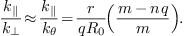 |
(327) |
Turbulence in tokamak plasmas usually has  , then
which is usually much smaller than unit for modes in
In the so-called high- approximation, the
poloidal harmonics of a mode is assumed to be arround  ,
which implies that
,
which implies that  and thus .
Consider a harmonic with poloidal mode number
and toroidal mode number ,
 |
(328) |
Choose a radial profile of the amplitude
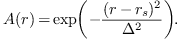 |
(329) |
Figure 35 plots the two-dimensional mode structures on the poloidal plane for two profiles of the radial phase variation given by
 |
(330) |
and
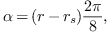 |
(331) |
respectively. Note that, compared with the case of  (no radial phase variation), the radial phase variation given by Eq. (331) influence the mode structure on the poloidal plane,
generating the so-called mode twist or shear[11], as shown
by the left figure of Fig. 35.
(no radial phase variation), the radial phase variation given by Eq. (331) influence the mode structure on the poloidal plane,
generating the so-called mode twist or shear[11], as shown
by the left figure of Fig. 35.
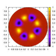 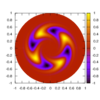 |
Figure 35. Two dimensional structure
(on |
Consider a mode composed of two poloidal harmonics
 |
(332) |
where  and
and  are the
poloidal mode number of the two poloidal harmonics. Consider the case
are the
poloidal mode number of the two poloidal harmonics. Consider the case
 . Then at the high field side of the midplane
 of
of  poloidal plane,
equation (332) is written
poloidal plane,
equation (332) is written
 |
(333) |
At the low field side of the midplane  of poloidal plane, equation (332) is
written
of poloidal plane, equation (332) is
written
 |
(334) |
Equations (333) and (334) indicates the amplitude of the mode at the low field side is larger than that at the strong field side, i.e., the mode exhibits a ballooning structure.
For a radial profile given by
 |
(335) |
and an initial phase , Figure 36
plots the two-dimensional structure of the mode on the poloidal plane.
The inital phase can have radial varation and
this has effects on the 2D structure of the mode. For instance, is chosen to be of the form
 |
(336) |
The resulting 2D mode structure is given in the right figure of Fig. 36, where the so-called mode shear can be seen[11].
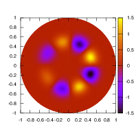 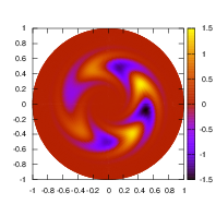 |
Figure 36. Two dimensional structure
(on |
to be done.
Using Eq. (65), we obtain
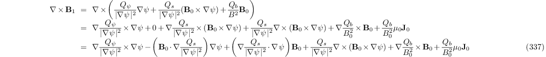
Using this, the second term on the right-hand side of Eq. (106) is written

The first term of Eq. (338) is written

The last equality is due to  . The second term of
Eq. (338) is written
. The second term of
Eq. (338) is written
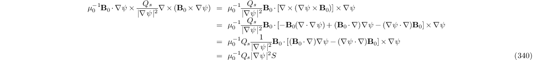
The last equality is due to that the coefficients before , i.e.,
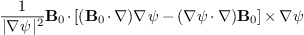
is equal to  (refer to Sec. 9.7 for
the proof). The third term of Eq. (338) is written
(refer to Sec. 9.7 for
the proof). The third term of Eq. (338) is written

Using Eqs. (339)-(341) in Eq. (338) yields
 |
(342) |
Now we calculate the  term appearing in Eq. (106), which can be written as
Gathering the terms involving in Eqs. (342)
and (343), we obtain
The second term of Eq. (344) is written

The last term of Eq. (344) is written

The terms in Eqs. (345) and (346) exactly cancel each other. Thus the expression in (344) now reduces to
 |
(347) |
Noting that

the expression (347) is further written as

where  is the unit vector along the direction of
equilibrium magnetic field, and is the magnetic
field curvature. Using these results, we obtain
is the unit vector along the direction of
equilibrium magnetic field, and is the magnetic
field curvature. Using these results, we obtain

Using the above results, the radial component equation
 |
(350) |
is written as
 |
(351) |
which can be arranged in the form

Define  , the above equation is written as

which is identical with Eq. (107).
In this subsection, we prove that

is zero.
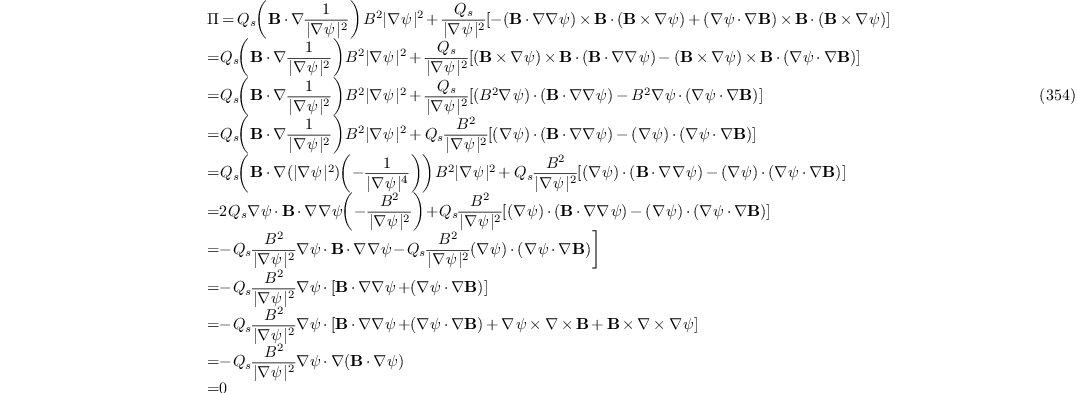
where the last second equality is due to the fact that

We want to prove that
 |
(356) |
where  . The right-hand side of Eq. (356)
is written as
. The right-hand side of Eq. (356)
is written as
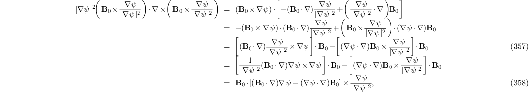
which is exactly the left-hand side of Eq. (356). Thus Eq. (356) is proved.
Try to prove that

Proof:
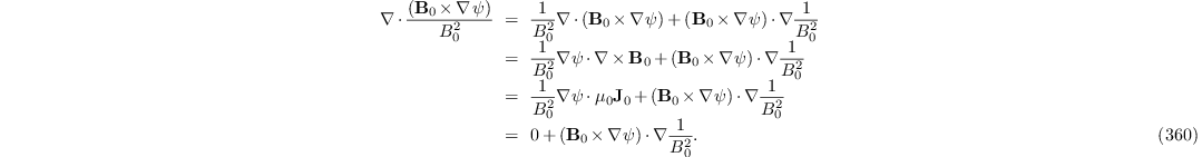
Using
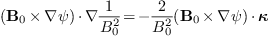 |
(361) |
(proof of this is given in Sec. 9.9), Eq. (360) is written as
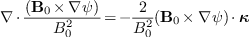 |
(362) |

The left-hand side of the equation is written as

Using  , the above equation is reduced to
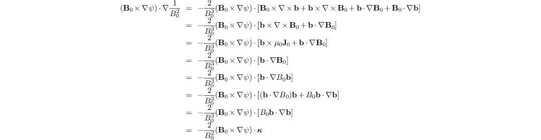
Another way to prove that  is equal to
  : The difference of these two terms is
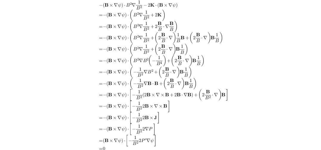
Thus we prove that
 |
(364) |
Try to prove that
 |
(365) |
Proof: We have
 |
(366) |
Thus

The last term on the right-hand side of Eq. (367) is written as

Using this, Eq. (367) is written as

i.e.,

thus Eq. (365) is proved.
The continuity equation can be written
 |
(370) |
which can be further written as
 |
(371) |
Then the incompressible condition  reduces to
 |
(372) |
On the other hand, equation (15) indicates that
 |
(373) |
which indicates that for incompressible plasma  .
.
[1] T. J. M. Boyd and J. J. Sanderson. The Physics of Plasmas. Cambridge University Press, Cambridge, UK, 2003.
[2] D. A. Gurnett and A. Bhattacharjee. Introduction to plasma physics : with space and laboratory applications. Cambridge University Press, Cambridge, UK, 2004.
[3] C.Z Cheng and M.S Chance. Nova: A nonvariational code for solving the mhd stability of axisymmetric toroidal plasmas. J. of Comput. Phys., 71(1):124 – 146, 1987.
[4] C. Z. Cheng. Kinetic extensions of magnetohydrodynamics for axisymmetric toroidal plasmas. Physics Reports, 211(1):1 – 51, 1992.
[5] W. H. Press, S. A. Teukolsky, W. T. Vetterling, and B. P. Flannery. Numerical Recipes in Fortran 77. Cambridge University Press, Cambridge, UK, 1992.
[6] W. Deng, Z. Lin, I. Holod, Z. Wang, Y. Xiao, and H. Zhang. Linear properties of reversed shear alfven eigenmodes in the diii-d tokamak. Nucl. Fusion, 52(4):043006, 2012.
[7] M. S. Chu, J. M. Greene, L. L. Lao, A. D. Turnbull, and M. S. Chance. A numerical study of the high-n shear alfv[e-acute]n spectrum gap and the high-n gap mode. Phys. Fluids B, 4(11):3713–3721, 1992.
[8] Youjun Hu, Guoqiang Li, N. N. Gorelenkov, Huishan Cai, Wenjun Yang, Deng Zhou, and Qilong Ren. Numerical study of alfvén eigenmodes in the experimental advanced superconducting tokamak. Physics of Plasmas (1994-present), 21(5):052510, 2014.
[9] G Q Li, Q L Ren, J P Qian, L L Lao, S Y Ding, Y J Chen, Z X Liu, B Lu, and Q Zang. Kinetic equilibrium reconstruction on east tokamak. Plasma Phys. Controlled Fusion, 55(12):125008, 2013.
[10] G. Y. Fu, C. Z. Cheng, R. Budny, Z. Chang, D. S. Darrow, E. Fredrickson, E. Mazzucato, R. Nazikian, K. L. Wong, and S. Zweben. Analysis of alpha particle driven toroidal alfv¨¦n eigenmodes in tokamak fusion test reactor deuterium tritium experiments. Phys. Plasmas, 3(11):4036, 1996.
[11] B. J. Tobias, I. G. J. Classen, C. W. Domier, W. W. Heidbrink, N. C. Luhmann, R. Nazikian, H. K. Park, D. A. Spong, and M. A. Van Zeeland. Fast ion induced shearing of 2d alfvén eigenmodes measured by electron cyclotron emission imaging. Phys. Rev. Lett., 106:075003, Feb 2011.
 Alfven continua (left) and sound continua (right) in the
cylindrical geometry limit for
Alfven continua (left) and sound continua (right) in the
cylindrical geometry limit for  , and
, and  (calculated by using Eqs. (
 in toroidal geometry depends on the poloidal angle,
the average value of
in toroidal geometry depends on the poloidal angle,
the average value of 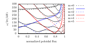
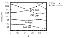
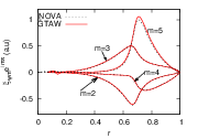
 ) of a
  . The equilibrium
is given by Eqs. (
. The equilibrium
is given by Eqs. (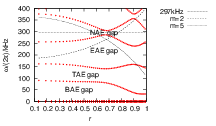
 and
and  continua in
cylindrical limit.
continua in
cylindrical limit.
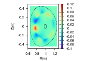
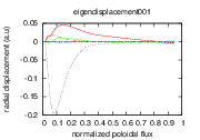
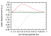
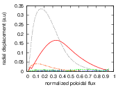
 .
The dominant poloidal harmonics are those with
.
The dominant poloidal harmonics are those with  and
and  . The equilibrium is given by Eqs. (
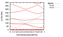
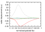
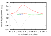
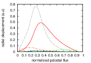
 .
The dominant poloidal harmonics are those with
.
The dominant poloidal harmonics are those with 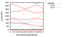
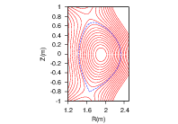
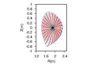
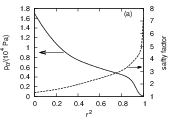
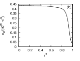
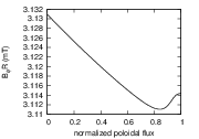
 as a function of the poloidal angle.
The different lines correspond to different magnetic surfaces. The
equilibrium is for EAST shot #38300 at 3.9s.
as a function of the poloidal angle.
The different lines correspond to different magnetic surfaces. The
equilibrium is for EAST shot #38300 at 3.9s.
 as a function
of the poloidal angle. The different lines correspond to the
values of
as a function
of the poloidal angle. The different lines correspond to the
values of 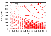

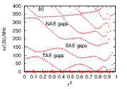
 approximation of the continua. Other parameters: toroidal mode
number
approximation of the continua. Other parameters: toroidal mode
number  . The
equilibrium used for this calculation is for EAST shot 38300 at
3.9s.
. The
equilibrium used for this calculation is for EAST shot 38300 at
3.9s.
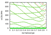
 (solid circles) and those obtained
when the truncation region is
(solid circles) and those obtained
when the truncation region is  (cross
marks). The equilibrium used for this calculation is for EAST shot
#38300 at 3.9s.
(cross
marks). The equilibrium used for this calculation is for EAST shot
#38300 at 3.9s.
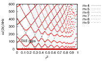
 Alfven continua (in slow sound approximation). The poloidal
harmonic numbers are truncated in the range
Alfven continua (in slow sound approximation). The poloidal
harmonic numbers are truncated in the range  .
The equilibrium used for this calculation is for EAST shot 38300
at 3.9s. The corresponding Alfven continua in the cylindrical
limit are also plotted.
.
The equilibrium used for this calculation is for EAST shot 38300
at 3.9s. The corresponding Alfven continua in the cylindrical
limit are also plotted.
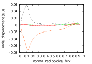
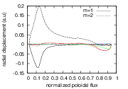
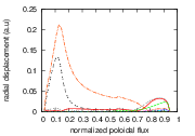
 .
The poloidal harmonics with
.
The poloidal harmonics with  and
and 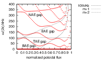
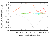
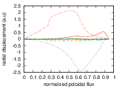
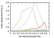
 .
The poloidal harmonics with
.
The poloidal harmonics with 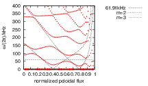
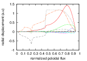
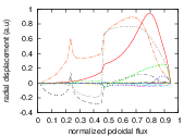
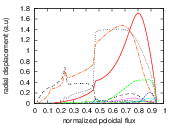
 .
The equilibrium is for EAST shot 38300 at 3.9s (G-file name:
g038300.03900). (D)
.
The equilibrium is for EAST shot 38300 at 3.9s (G-file name:
g038300.03900). (D)
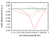
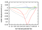
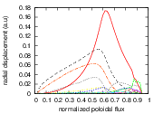
 . The equilibrium is for EAST shot
38300 at 3.9s (G-file name: g038300.03900). (D)
. The equilibrium is for EAST shot
38300 at 3.9s (G-file name: g038300.03900). (D)
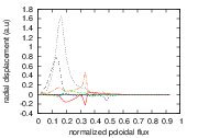
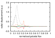
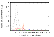
 .
The poloidal harmonics with
.
The poloidal harmonics with  are dominant. The poloidal harmonics are truncated
into the range
are dominant. The poloidal harmonics are truncated
into the range  in the numerical
calculation. The equilibrium is for EAST shot 38300 at 3.9s
(G-file name: g038300.03900). (H)
in the numerical
calculation. The equilibrium is for EAST shot 38300 at 3.9s
(G-file name: g038300.03900). (H)
 calculated by Eq. (
 (calculated by Eq. (
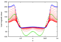
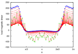
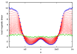
 (right)
as a function of the poloidal angle. The different lines
corresponds to the shear on different magnetic surfaces. The stars
correspond to the values of the shear on the boundary magnetic
surface while the plus signs correspond to the value on the
innermost magnetic surface (the magnetic surface adjacent to the
magnetic axis). The equilibrium is a Solovev equilibrium.
(right)
as a function of the poloidal angle. The different lines
corresponds to the shear on different magnetic surfaces. The stars
correspond to the values of the shear on the boundary magnetic
surface while the plus signs correspond to the value on the
innermost magnetic surface (the magnetic surface adjacent to the
magnetic axis). The equilibrium is a Solovev equilibrium.
 (solid line) and
  (plus mark) as a function
of the radial coordinate
(plus mark) as a function
of the radial coordinate  (
( plane) given by Eqs. (
 ,
,  ,
,  .
Left figure is for
.
Left figure is for  and right figure is for
 given by Eq. (
 coordinate is at
the low-field-side of the midplane and the positive direction is
in the anti-clockwise direction). A GIF animation of the time
evolution of the mode can be found at
http://theory.ipp.ac.cn/~yj/figures/mode_rotation3.gif
coordinate is at
the low-field-side of the midplane and the positive direction is
in the anti-clockwise direction). A GIF animation of the time
evolution of the mode can be found at
http://theory.ipp.ac.cn/~yj/figures/mode_rotation3.gif
 ,
,