| Nonlinear gyrokinetic
equation |
|
Institute of Plasma Physics, Chinese Academy of
Sciences
Email: yjhu@ipp.cas.cn
|
|
|
The nonlinear  gyrokinetic
equation in Frieman-Chen's paper[3] is re-derived, with
more details provided. All formulas are in SI units. Numerical
implementation of the gyrokinetic model using the PIC method is also
discussed. A gyrokinetic PIC code called TEK was developed
using the formulas given in this document. TEK has been benchmarked
with GENE code in the DIII-D cyclone base case for both ITG-KBM
transition and ITG-TEM transition.
gyrokinetic
equation in Frieman-Chen's paper[3] is re-derived, with
more details provided. All formulas are in SI units. Numerical
implementation of the gyrokinetic model using the PIC method is also
discussed. A gyrokinetic PIC code called TEK was developed
using the formulas given in this document. TEK has been benchmarked
with GENE code in the DIII-D cyclone base case for both ITG-KBM
transition and ITG-TEM transition.
1Introduction
1.1Gyrokinetic?
Electromagnetic perturbations of frequency lower than the ion cyclotron
frequency are widely believed to be more important than high-frequency
ones in transporting plasma in tokamaks. (This assumption can be
verified numerically when we are able to do a full simulation including
both low-frequency and high-frequency perturbations. This kind of
verification is not possible at present due to computation costs.)
If we assume that only low-frequency perturbations are present, the
Vlasov equation can be simplified. Specifically, symmetry of the
particle distribution function in the phase space can be established if
we choose suitable phase-space coordinates and split the distribution
function in a proper way. The symmetry is along the so-called gyro-angle
 in the guiding-center coordinates
  . In obtaining the equation for the gyro-angle
independent part of the distribution function, we need to average the
equation over the gyro-angle and thus this model
is called “gyrokinetic”.
. In obtaining the equation for the gyro-angle
independent part of the distribution function, we need to average the
equation over the gyro-angle and thus this model
is called “gyrokinetic”.
In deriving the gyrokinetic equation, the perturbed electromagnetic
field is assumed to be known and of low-frequency. To do a kinetic
simulation, we need to solve Maxwell's equations to obtain the perturbed
electromagnetic field. It is still possible that high frequency modes
(e.g., compressional Alfven waves and  modes)
appear in a gyrokinetic simulation. If the amplitude of high frequency
modes is significantly large, then the simulation is invalid because the
gyrokinetic model is invalid in this case.
modes)
appear in a gyrokinetic simulation. If the amplitude of high frequency
modes is significantly large, then the simulation is invalid because the
gyrokinetic model is invalid in this case.
Our starting point is the Vlasov equation in terms of particle
coordinates  :
:
 |
(1) |
where  is the particle distribution function,
 and
and  are the location and
velocity of particles. The distribution function
are the location and
velocity of particles. The distribution function  depends on 6 phase-space variables ,
besides the time
depends on 6 phase-space variables ,
besides the time  .
.
1.2Guiding-center coordinates: a
simple example
Choose Cartesian coordinates  for the
configuration space .
Consider a simple case where the electromagnetic field is a
time-independent field given by
for the
configuration space .
Consider a simple case where the electromagnetic field is a
time-independent field given by  and
and  . Let us examine the Vlasov equation in this
case and see whether there is any coordinate system that can simplify
the Vlasov equation.
. Let us examine the Vlasov equation in this
case and see whether there is any coordinate system that can simplify
the Vlasov equation.
Describe the velocity space using a right-handed cylindrical
coordinates  , where
  ,
,  is the
unit vector along the magnetic field, is the
azimuthal angle of the perpendicular velocity (
is the
unit vector along the magnetic field, is the
azimuthal angle of the perpendicular velocity ( ) relative to
  .
Note that these coordinates are defined relative to the local magnetic
field, which, in more general cases, may vary in space.
.
Note that these coordinates are defined relative to the local magnetic
field, which, in more general cases, may vary in space.
Next, let us express the spatial gradient of in
terms of partial derivatives:
 |
(2) |
Note that this gradient is taken by holding
constant (i.e.,  constant rather than constant). So, we need do the following coordinate
transform:
constant rather than constant). So, we need do the following coordinate
transform:
 |
(3) |
Using chain rule, expression (2) is written as
Note that the partial derivatives
 |
(6) |
are generally nonzero since the defintion of
depends on the local magnetic field direction. In our simple case, they
are zero since the magnetic field direction is uniform. Similarly, we
obtain
 |
(7) |
 |
(8) |
Then, in  coordinates, the spatial gradient of
is written as
coordinates, the spatial gradient of
is written as
 |
(9) |
Next, consider the gradient in velocity space
where  ,
,  , and
, and  .
Using Eq. (10),
.
Using Eq. (10),  is written as
where  is the gyro-frequency. Then the Vlasov
equation (1) is written as
is the gyro-frequency. Then the Vlasov
equation (1) is written as
 |
(12) |
i.e.,
 |
(13) |
Define the following coordinates transform (guiding-center transform):
 |
(14) |
Next, we express the partial derivatives of
appearing in Eq. (13) in terms of the guiding-center
coordinates. Using the chain rule, we obtain
Similarly, for other derivatives, we obtain
 |
(16) |
and
where we have assumed that the dependence of  and
and
 on
on  (via
(via  ) is weak enough to be neglected. And also
 |
(19) |
Using the above results, equation (13) in the
guiding-center coordinates is written as
 |
(20) |
Here we find some terms cancel each other, giving
 |
(21) |
Equation (21) is the equation for
in the guiding-center coordinates  .
.
1.2.1Gyro-averaging
Define gyro-phase averaging operator
 |
(22) |
Then averaging Eq. (21) over  ,
we get
,
we get
 |
(23) |
As is assumed above, is approximately
independent of and thus
in Eq. (23) can be moved outside of the gyro-angle
integration, giving
 |
(24) |
Peforming the integration, we get
 |
(25) |
Since  and
and  correspond to
the same phase space location, the corresponding values of the
distribution function must be equal. Then the above equation reduces to
correspond to
the same phase space location, the corresponding values of the
distribution function must be equal. Then the above equation reduces to
 |
(26) |
which is an equation for the gyro-angle independent part of the
distribution function.
Next let us investigate whether the guiding-center transform can be made
use of to simplify the kinetic equation for more general cases where we
have a (weakly) non-uniform static magnetic field, plus electromagnetic
perturbations of low frequency (and of small amplitude and  ). And we will include the effect that
  depends on ,
i.e., grad-B and curvature drift.
depends on ,
i.e., grad-B and curvature drift.
2Transform Vlasov equation from particle
coordinates to guiding-center coordinates
Next, we define the guiding-center transform and then transform the
Vlasov equation from the particle coordinates  to
the guiding-center coordinates. The main task is to express the gradient
operators
to
the guiding-center coordinates. The main task is to express the gradient
operators  and
and  in terms
of the guiding-center coordinates.
in terms
of the guiding-center coordinates.
2.1Guiding-center transformation
In a magnetic field, given a particle location and velocity , we know how to calculate its guiding-center
location  :
:
 |
(27) |
where  ,
,  ,
,  is the equilibrium
(macroscopic) magnetic field at the particle position. We will consider
Eq. (27) as a transform and call it guiding-center
transform. Note that the transform (27) involves both
position and velocity of particles.
is the equilibrium
(macroscopic) magnetic field at the particle position. We will consider
Eq. (27) as a transform and call it guiding-center
transform. Note that the transform (27) involves both
position and velocity of particles.
Given , it is straightforward
to obtain  by using Eq. (27). On the
other hand, the inverse transform (i.e., given
by using Eq. (27). On the
other hand, the inverse transform (i.e., given  , to find )
is not easy because and
, to find )
is not easy because and  depend on , which usually
requires us to solve a nonlinear equation for its root. Numerically, one
can use
depend on , which usually
requires us to solve a nonlinear equation for its root. Numerically, one
can use
 |
(28) |
as an iteration scheme to compute ,
with the initial guess chosen as  .
If we stop at the first iteration, then
.
If we stop at the first iteration, then
 |
(29) |
The approximation relation (29) is usually used as the
inverse guiding-center transformation in gyrokinetic PIC simulations.
This transformation needs to be performed numerically when we deposit
markers to grids, or when we calculate the gyro-averaged field to be
used in pushing guiding-centers.
The equilibrium magnetic field we will consider has spatial scale length
much larger than the thermal gyro radius. In this case the difference
between the values of  and the corresponding
values at the guiding-center location
and the corresponding
values at the guiding-center location  is
negligible. The difference between equilibrium field values evaluated at
and is neglected in
gyrokinetic theory (except in deriving the gradient/curvature drift).
Therefore it does not matter whether the above
is
negligible. The difference between equilibrium field values evaluated at
and is neglected in
gyrokinetic theory (except in deriving the gradient/curvature drift).
Therefore it does not matter whether the above  is evaluated at or .
What matters is where the perturbed fields are evaluated: at or at . The
values of perturbed fields at and the
corresponding guiding-center location are
different. This is the origin of the finite Larmor radius (FLR) effect.
is evaluated at or .
What matters is where the perturbed fields are evaluated: at or at . The
values of perturbed fields at and the
corresponding guiding-center location are
different. This is the origin of the finite Larmor radius (FLR) effect.
For later use, define  , which
is the vector gyro-radius pointing from the the guiding-center to the
particle position.
, which
is the vector gyro-radius pointing from the the guiding-center to the
particle position.
2.2Choosing velocity coordinates
The guiding-center transformations (27) and (29)
involve the particle velocity .
It is the cross product between and  that is actually used. Therefore, only the perpendicular
velocity (which is defined by
that is actually used. Therefore, only the perpendicular
velocity (which is defined by  )
enters the transform. A natural choice of coordinates for the
perpendicular velocity is
)
enters the transform. A natural choice of coordinates for the
perpendicular velocity is  ,
where
,
where  and is the
azimuthal angle of the perpendicular velocity in the local perpendicular
plane. There are degrees of freedom in choosing one of the two
perpendicular basis vectors, with respect to which
is defined. In GEM code, one of the perpendicular direction is
chosen as the direction perpendicular to the magnetic surface, which is
fully determined at each spatial point. (We need to define the
perpendicular direction at each spatial location to make
and is the
azimuthal angle of the perpendicular velocity in the local perpendicular
plane. There are degrees of freedom in choosing one of the two
perpendicular basis vectors, with respect to which
is defined. In GEM code, one of the perpendicular direction is
chosen as the direction perpendicular to the magnetic surface, which is
fully determined at each spatial point. (We need to define the
perpendicular direction at each spatial location to make  defined, which is needed in the Vlasov differential
operators. However, it seems that terms related to
are finally dropped due to that they are of higher order**check.)
defined, which is needed in the Vlasov differential
operators. However, it seems that terms related to
are finally dropped due to that they are of higher order**check.)
In the following, will be called
“gyro-angle”. Note that is a
coordinate of space. In particle coordinate
, by definition, varying does not affect .
In the guiding-center coordinates  ,
by definition, varying does not affect . However, when transformed back to
particle coordinates, affects both the velocity
coordinate and the spatial coordinate. [Consider a series of points in
terms of guiding-center coordinates with
,
by definition, varying does not affect . However, when transformed back to
particle coordinates, affects both the velocity
coordinate and the spatial coordinate. [Consider a series of points in
terms of guiding-center coordinates with  fixed but with changing.
Using the inverse guiding-center transform (29), we know
that the above points form a gyro-ring in space, i.e.,
influences spatial location, in addtion to velocity.]
fixed but with changing.
Using the inverse guiding-center transform (29), we know
that the above points form a gyro-ring in space, i.e.,
influences spatial location, in addtion to velocity.]
The gyro-angle is an important variable we will stick to because we need
to directly perform averaging over this variable (with
fixed) in deriving the gyrokinetic equation. We have multiple options
for the remaining velocity coordinates , such as  , or
, or  , or
, or
 . In Frieman-Chen's paper,
the velocity coordinates other than are chosen
to be
. In Frieman-Chen's paper,
the velocity coordinates other than are chosen
to be  defined by
 |
(30) |
and
 |
(31) |
where  is the equilibrium (macroscopic)
electrical potential. Choosing
is the equilibrium (macroscopic)
electrical potential. Choosing  as one of the
phase space coordinates is nontrivial because it turns out to be a
constant of motion. And this choice seems to be important in sucessfully
getting the final gyrokinetic equation (I need to check this).
as one of the
phase space coordinates is nontrivial because it turns out to be a
constant of motion. And this choice seems to be important in sucessfully
getting the final gyrokinetic equation (I need to check this).
Note that  is not sufficient in uniquely
determining a velocity vector. An additional parameter
is not sufficient in uniquely
determining a velocity vector. An additional parameter  is needed to determine the sign of .
In the following, the dependence of the distribution function on
is needed to determine the sign of .
In the following, the dependence of the distribution function on  is often not explicitly shown in the variable list
(i.e., is hidden/suppressed), which, however,
does not mean that the distribution function is independent of .
is often not explicitly shown in the variable list
(i.e., is hidden/suppressed), which, however,
does not mean that the distribution function is independent of .
Another frequently used velocity coordinates are  . In the following, I will derive the gyrokinetic
equation in coordinates. After that, I transform
it to coordinates.
. In the following, I will derive the gyrokinetic
equation in coordinates. After that, I transform
it to coordinates.
One important thing to note about the above velocity coordinates is that
they are defined relative to the local magnetic field. Because the
tokamak magnetic field is spatially varying, the above velocity
coordinates are also spatially varying for a fixed velocity  . Specifically, the following derivatives are
nonzero:
. Specifically, the following derivatives are
nonzero:
 |
(32) |
2.3Summary of the phase-space coordinate
transform
The transform from particle variables to
guiding-center variables  is given by
 |
(33) |
As mentioned above, the dependence of the distribution function on will be hidden in the following.
2.4Distribution function in terms of
guiding-center variables
Denote the particle distribution function expressed in particle
coordinates by  ,
and the same distribution expressed in the guiding-center variables
,
and the same distribution expressed in the guiding-center variables  by
by  . Then
 |
(34) |
where and are related to
each other by the guiding-center transform (29). Equation
(34) along the guiding-center transform can be considered
as the definition of .
As is conventionally adopted in multi-variables calculus, both and are often denoted by the same
symbol, say . Which set of
independent variables are actually assumed is inferred from the context.
This is one subtle thing for gyrokinetic theory in particular and for
multi-variables calculus in general. (Sometimes, it may be better to use
subscript notation on to identify which
coordinates are assumed. One example where this distinguishing is
important is encountered when we try to express the diamagnetic flow in
terms of , which is discussed
in Appendix F.)
In practice, is often called the guiding-center
distribution function whereas is called the
particle distribution function. However, they are actually the same
distribution function expressed in different variables. The name
“guiding-center distribution function” is misleading because
it may imply that we can count the number of guiding-centers to obtain
this distribution function but this implication is wrong.
2.5Spatial gradient operator in guiding-center
coordinates
Using the chain-rule, the spatial gradient  is
written
is
written
 |
(35) |
From the definition of , Eq.
(27), we obtain
 |
(36) |
where  is the unit dyad. From the definition of
 , we obtain
 |
(37) |
where  . Using the above
results, equation (35) is written as
. Using the above
results, equation (35) is written as
 |
(38) |
As mentioned above, the partial derivative is
taken by holding constant. Since is spatially varying,  is spatially
varying when holding constant. Therefore
is spatially
varying when holding constant. Therefore  and
and  are generally nonzero.
The explicit expressions of these two derivatives are needed later in
the derivation of the gyrokinetic equation and is discussed in Appendix
I. For notation ease, define
are generally nonzero.
The explicit expressions of these two derivatives are needed later in
the derivation of the gyrokinetic equation and is discussed in Appendix
I. For notation ease, define
 |
(39) |
and
 |
(40) |
then expression (38) is written as
 |
(41) |
Note that  is a shorthand for

i.e., it is taken by holding constant (rather
than holding constant). For notation ease, is sometimes denoted by  or
simply
or
simply  .
.
2.6Velocity gradient operator in
guiding-center coordinates
Next, let us express the velocity gradient  in
terms of the guiding-center variables. Using the chain rule, is written
in
terms of the guiding-center variables. Using the chain rule, is written
 |
(42) |
From the definition of , we
obtain
From the definition of , we
obtain
 |
(44) |
From the definition of , we
obtain
 |
(45) |
From the definition of , we
obtain
 |
(46) |
where  is defined by
 |
(47) |
Using the above results, expression (42) is written
 |
(48) |
2.7Time derivatives in guiding-center
coordinates
In terms of the guiding-center variables, the time partial derivative
 appearing in Vlasov equation is written as
 |
(49) |
where  . Here
  and
and  are not necessarily zero because the
equilibrium quantities involved in the definition of the guiding-center
transformation are in general time dependent. This time dependence is
assumed to be very slow in the gyrokinetic ordering discussed later. In
the following, and will
be dropped, i.e.,
are not necessarily zero because the
equilibrium quantities involved in the definition of the guiding-center
transformation are in general time dependent. This time dependence is
assumed to be very slow in the gyrokinetic ordering discussed later. In
the following, and will
be dropped, i.e.,
 |
(50) |
2.8Final form of Vlasov equation in
guiding-center coordinates
Using the above results, the Vlasov equation in guiding-center
coordinates is written
Using tensor identity  ,
equation (51) is written as
,
equation (51) is written as
This is the Vlasov equation in guiding-center coordinates.
3 form of Vlasov
equation in guiding-center variables
form of Vlasov
equation in guiding-center variables
3.1Electromagnetic field perturbation
Since the definition of the guiding-center variables
involves the equilibrium fields and  , to further simplify Eq. (52), we
need to separate electromagnetic field into equilibrium and perturbation
parts. Writing the electromagnetic field as
, to further simplify Eq. (52), we
need to separate electromagnetic field into equilibrium and perturbation
parts. Writing the electromagnetic field as
 |
(53) |
and
 |
(54) |
then substituting these expressions into equation (52) and
moving all terms involving the field perturbations to the right-hand
side, we obtain
where  is defined by
Next, let us simplify the left-hand side of Eq. (55). Note
that
Note that
 |
(58) |
where  is defined by
  , which is the
  drift.
Further note that
drift.
Further note that
which can be combined with  term, yielding
  .
.
Using Eqs. (58), (59), and (57),
the left-hand side of equation (55) is written as
where  is often called the unperturbed Vlasov
propagator in guiding-center coordinates .
is often called the unperturbed Vlasov
propagator in guiding-center coordinates .
[Equation (60), corresponds to Eq. (7) in Frieman-Chen's
paper[3]. In Frieman-Chen's equation (7), there is a term

where  is a given macroscopic electric field
introduced when defining the guiding-center transformation. In my
derivation is chosen to be equal to the
equilibrium electric field, and thus the above term is zero.]
is a given macroscopic electric field
introduced when defining the guiding-center transformation. In my
derivation is chosen to be equal to the
equilibrium electric field, and thus the above term is zero.]
Using the above results, Eq. (55) is written as
 |
(61) |
i.e.
It is instructive to consider some special cases of the above
complicated equation. Consider the case that the equilibrium magnetic
field is uniform and time-independent,  , and the electrostatic limit
  , then equation (62)
is simplified as
, then equation (62)
is simplified as
If neglecting the  perturbation, the above
equation reduces to
perturbation, the above
equation reduces to
 |
(65) |
which agrees with Eq. (21) discussed in Sec. 1.2.
3.2Distribution function perturbation
Expand the distribution function as
 |
(66) |
where  is assumed to be an equilibrium
distribution function, i.e.,
is assumed to be an equilibrium
distribution function, i.e.,
 |
(67) |
Using Eqs. (66) and (67) in Eq. (61),
we obtain an equation for  :
:
 |
(68) |
3.3Gyrokinetic ordering
To facilitate the simplification of the Vlasov equation in the
low-frequency regime, we assume the following orderings (some of which
are roughly based on experiment measure of fluctuations responsible for
tokamak plasma transport, some of which can be invalid in some
interesting cases.) These ordering are often called the standard
gyrokinetic orderings.
3.3.1Assumptions for equilibrium
quantities
Define the spatial scale length  of equilibrium
quantities by
of equilibrium
quantities by  . Assume that
is much larger than the thermal gyro-radius
. Assume that
is much larger than the thermal gyro-radius
 , i.e.,
  is a small parameter, where
  is the thermal
velocity. That is
is the thermal
velocity. That is
 |
(69) |
and
 |
(70) |
The equilibrium flow, which is given by
 |
(71) |
is assumed to be weak with
 |
(72) |
3.3.2Assumptions for perturbations
In terms of the scalar and vector potentials,  and
and  , the electromagnetic
perturbation is written as
, the electromagnetic
perturbation is written as
 |
(73) |
and
 |
(74) |
Most gyrokinetic simulations approximate the vector potential as  . Then Eq. (73) is
writen as
. Then Eq. (73) is
writen as
 |
(75) |
We assume that the amplitudes of perturbations are small:
 |
(76) |
Further we assume that the parallel wavelength of perturbations is much
longer than  :
:
 |
(77) |
and pependicular wavelength is of the same oder of :
 |
(78) |
Equation (75) indicates that  .
Then the odering in (76) indicates that
.
Then the odering in (76) indicates that  is of the same order of .
The electrical field perturbation is written as
 |
(79) |
 |
(80) |
Using the above orderings, it is ready to see that  is one order smaller than
  ,
i.e.,
,
i.e.,
 |
(81) |
We assume the perturbations are of low frequency:  , i.e.,
 |
(82) |
3.4Equation for macroscopic distribution
function
The evolution of the macroscopic quantity is
governed by Eq. (67), i.e.,
 |
(83) |
where the left-hand side is written as

Expand as  .,
where
.,
where  . Then, the balance on
order
. Then, the balance on
order  gives
gives
 |
(84) |
i.e.,  is independent of the gyro-angle . The balance on
  gives
gives
 |
(85) |
Performing averaging over ,
 , on the above equation and
noting that is independent of , we obtain
, on the above equation and
noting that is independent of , we obtain
 |
(86) |
Note that a quantity  that is independent of will depend on when
transformed to guiding-center coordinates, i.e.,
that is independent of will depend on when
transformed to guiding-center coordinates, i.e.,  . Therefore
  depends on
gyro-angle . However, since
depends on
gyro-angle . However, since
 for equilibrium quantities, the gyro-angle
dependence of the equilibrium quantities can be neglected. Specifically,
,
for equilibrium quantities, the gyro-angle
dependence of the equilibrium quantities can be neglected. Specifically,
,  and
can be considered to be independent of . As to
and
can be considered to be independent of . As to  , we have
  .
Since is considered independent of , so does .
Using these results, equation (86) is written
.
Since is considered independent of , so does .
Using these results, equation (86) is written
 |
(87) |
Using  , the above equation is
written as
, the above equation is
written as
 |
(88) |
Note that
 |
(89) |
where the error is of  , and
thus, accurate to
, and
thus, accurate to  , the last
term of equation (88) is zero. Then equation (88)
is written as
, the last
term of equation (88) is zero. Then equation (88)
is written as
 |
(90) |
which implies that is constant along a magnetic
field line.
3.5Equation for
Using  , equation (68)
is written as
, equation (68)
is written as
 |
(91) |
where  is a nonlinear term which is of order
  or higher,
  and
and  are linear terms which are of order
or higher. The linear term is given by
are linear terms which are of order
or higher. The linear term is given by
 |
(92) |
In obtaining (92), use has been made of  . Another linear term
is written as
. Another linear term
is written as
where  is of order and
all the other terms are of order .
is of order and
all the other terms are of order .
Next, to reduce the complexity of algebra, we consider the easier case
in which  .
.
3.5.1Balance on order : adiabatic response
The balance between the leading terms (terms of ) in Eq. (91) requires that
 |
(94) |
where  is a unknown distribution function to be
solved from the above equation. It is ready to verify that
is a unknown distribution function to be
solved from the above equation. It is ready to verify that
 |
(95) |
is a solution to the above equation, accurate to . [Proof: Substitute expression (95)
into the left-hand side of Eq. (94), we obtain
Using
Eq. (96) is written as
where terms of have been dropped. Similarly,
dropping the parallel electric field term (which is of ) on the right-hand side of Eq. (94),
we find it is identical to the right-hand side of Eq. (99)]
3.5.2Separate into
adiabatic and non-adiabatic part
As is discussed above, the terms of can be
eliminated by splitting a so-called adiabatic term form . Specifically, write
as
 |
(100) |
where is given by (95), i.e.,
 |
(101) |
which depends on the gyro-angle via and this
term is often called adiabatic term. Plugging expression (100)
into equation (91), we obtain
 |
(102) |
Next, let us simplify the linear term on the right-hand side, i.e,  , (which should be of or higher because
  cancels all the
terms in ).
cancels all the
terms in ).
 is written
where the error is of order  .
In obtaining the above expression, use has been made of
.
In obtaining the above expression, use has been made of  ,
,  ,
, , and the definition of
,
, , and the definition of  and
and
 given in expressions (39) and (40). The expression (103) involves operated by the Vlasov propagator
  . Since takes the most
simple form when expressed in particle coordinates (if in guiding-center
coordinates,
. Since takes the most
simple form when expressed in particle coordinates (if in guiding-center
coordinates,  , which depends
on velocity coordinates and thus more complicated), it is convenient to
use the Vlasov propagator expressed in particle
coordinates. Transforming back to the particle
coordinates, expression (103) is written
, which depends
on velocity coordinates and thus more complicated), it is convenient to
use the Vlasov propagator expressed in particle
coordinates. Transforming back to the particle
coordinates, expression (103) is written
Using this and expression (92),  is
written as
is
written as
where the two terms of (the terms in blue and red) cancel each other, with
the remain terms being all of ,
i.e, the contribution of the adiabatic term cancels the leading order
terms of on the RHS of Eq. (102).
The consequence of this is that, as we will see in Sec. 3.6.1,
 is independent of the gyro-angle, accurate to
order . Therefore, separating
is independent of the gyro-angle, accurate to
order . Therefore, separating
 into adiabatic and non-adiabatic parts also
corresponds to separating into gyro-angle
dependent and gyro-angle independent parts.
into adiabatic and non-adiabatic parts also
corresponds to separating into gyro-angle
dependent and gyro-angle independent parts.
3.5.3Linear term expressed in terms of and
Let us rewrite the linear term (107) in terms of and . The  term in expression (107) is written as
 |
(108) |
Note that this term needs to be accurate to only . Then
 |
(109) |
where the error is of . Using
the vector identity  and noting
is constant for
and noting
is constant for  operator, the above equation is
written
operator, the above equation is
written
 |
(110) |
Note that Eq. (41) indicates that  , where the error is of , then the above equation is written
 |
(111) |
Further note that the parallel gradients in the above equation are of
and thus can be dropped. Then expression (111) is written
where  is defined by
 |
(113) |
Using expression (112), equation (107) is
written
 |
(114) |
where all terms are of .
3.6Equation for the non-adiabatic part
Plugging expression (114) into Eq. (102), we
obtain
 |
(115) |
where is given by Eq. (93), i.e.,
3.6.1Expansion of
Expand as

where  , and note that the
right-hand side of Eq. (115) is of , then, the balance on order
requires
, and note that the
right-hand side of Eq. (115) is of , then, the balance on order
requires
 |
(117) |
i.e.,  is gyro-phase independent.
The balance on order requires (for the special
case of  ):
):
3.6.2Gyro-averaging
Define the gyro-average operator  by
by
 |
(119) |
where  is an arbitrary function of guiding-center
variables. The gyro-averaging is an integration in the velocity space.
[For a field quantity, which is independent of the velocity in particle
coordinates, i.e.,
is an arbitrary function of guiding-center
variables. The gyro-averaging is an integration in the velocity space.
[For a field quantity, which is independent of the velocity in particle
coordinates, i.e.,  , it is
ready to see that the above averaging is a spatial averaging over a
gyro-ring.]
, it is
ready to see that the above averaging is a spatial averaging over a
gyro-ring.]
Gyro-averaging Eq. (118), we obtain
|
|
 |
|
|
|
 |
(120) |
where use has been made of  ,
where the error is of order higher than .
Note that . Since is approximately independent of , so does .
Using this, the first gyro-averaging on the left-hand side of the above
equation is written
,
where the error is of order higher than .
Note that . Since is approximately independent of , so does .
Using this, the first gyro-averaging on the left-hand side of the above
equation is written
 |
(121) |
The second gyro-averaging on the left-hand side of Eq. (120)
can be written as
 |
(122) |
where  is the magnetic curvature and gradient
drift (Eq. (122) is derived in Appendix xx, to do later).
Then Eq. (120) is written
is the magnetic curvature and gradient
drift (Eq. (122) is derived in Appendix xx, to do later).
Then Eq. (120) is written
|
|
 |
|
|
|
 |
(123) |
3.6.3Simplification of the nonlinear term
Next, we try to simplify the nonlinear term  appearing in Eq. (123), which is written as
First, let us focus on the first term, which can be written as
Using the above results, the nonlinear term  is
written as
is
written as
 |
(126) |
Accurate to  the first term on
the right-hand side of the above is zero. [Proof:
the first term on
the right-hand side of the above is zero. [Proof:
where use has been made of  ,
where the error is of . Using
the above results, expression (126) is written as
,
where the error is of . Using
the above results, expression (126) is written as
 |
(128) |
Using the expression of given by Eq. (56),
the above expression is written as
where use has been made of  .
Using Eq. (112), we obtain
.
Using Eq. (112), we obtain
 |
(130) |
The other two terms in Eq. (129) can be proved to be zero.
[Proof:
] Using the above results, the nonlinear term is finally written as
 |
(133) |
Using this in Eq. (128), we obtain
 |
(134) |
which is of .
3.6.4Final equation for the non-adiabatic part
of distribution function perturbation
Using the above results, the gyro-averaged kinetic equation for is finally written as
|
|
 |
|
|
|
 |
(135) |
where  is gyro-angle independent and is related
to the distribution function perturbation by
is gyro-angle independent and is related
to the distribution function perturbation by
 |
(136) |
where the first term is called “adiabatic
part”, which depends on the gyro-phase via
. (Equation (135)
is the special case ( ) of the
Frieman-Chen nonlinear gyrokinetic equation given in Ref. [3].
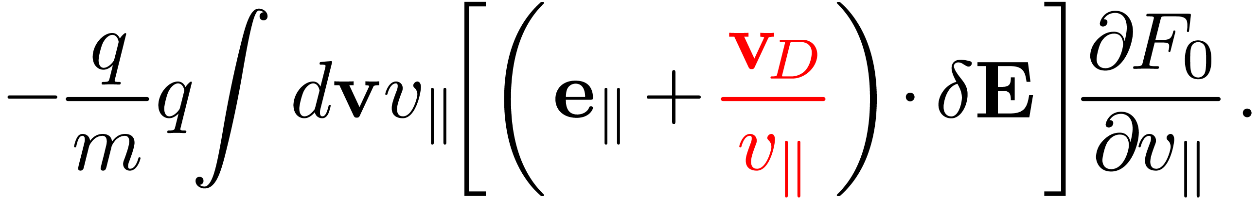
Note that the nonlinear terms only appear on the left-hand side of Eq.
(135) and all the terms on the right-hand side are linear.)
Here is the guiding-center drift velocity in the
equilibrim field;
) of the
Frieman-Chen nonlinear gyrokinetic equation given in Ref. [3].
Note that the nonlinear terms only appear on the left-hand side of Eq.
(135) and all the terms on the right-hand side are linear.)
Here is the guiding-center drift velocity in the
equilibrim field;  is the gyro-phase averaging
operator;
is the gyro-phase averaging
operator;  ; the term
 |
(137) |
consists of the  drift and magnetic fluttering
term (refer to expression (341) in Sec. C.3).
For notaiton ease, this term is denoted by
drift and magnetic fluttering
term (refer to expression (341) in Sec. C.3).
For notaiton ease, this term is denoted by  in
the following:
in
the following:
 |
(138) |
Note that  , which is the
gradient operator in the guiding-center coordinates
while holding constant. How do we numerically
calculate
, which is the
gradient operator in the guiding-center coordinates
while holding constant. How do we numerically
calculate  in PIC simulations? The difficulty is
that grid is not available, which makes it
difficult to use the finite difference method. Meanwhile grid is available in PIC simulations. It turns out we can
make use of grid to approximatly calculate the
derivatives in space. Using
in PIC simulations? The difficulty is
that grid is not available, which makes it
difficult to use the finite difference method. Meanwhile grid is available in PIC simulations. It turns out we can
make use of grid to approximatly calculate the
derivatives in space. Using  and the definition
  we obtain
which is accurate up to in gyrokinetic ordering.
The above relation indicates that the value of  at a guidng-center location is approximately equal to the value of
  at the corresponding particle position. Therefore we
can use defined on grid
to compute on gridpoints, and interpolate it to
the particle position and this is a good approximation of .
at the corresponding particle position. Therefore we
can use defined on grid
to compute on gridpoints, and interpolate it to
the particle position and this is a good approximation of .
Also note that  is not known on
grid (it is known at random markers). So, to calculate
is not known on
grid (it is known at random markers). So, to calculate  , we need to exchange the operation order:
 |
(140) |
For notation ease, the subscripts  and
and  are usually dropped. Which one is intended should be
obvious from the context.
are usually dropped. Which one is intended should be
obvious from the context.
4Gyrokinetic equation suitable for numerical
simulation
The gyrokinetic equation (135) contains time derivatives of
unknown and on the
right-hand side, which is problematic if treated by using explicit
finite difference in PIC simulations. Next, we discuss some methods that
can eliminate these terms, making the gyrokinetic equation more amenable
to PIC simulations.
4.1Eliminate  term on
the right-hand side of Eq. (135)
term on
the right-hand side of Eq. (135)
The coefficient before  in Eq. (135)
involves the time derivative of
in Eq. (135)
involves the time derivative of  ,
which is problematic if treated by using explicit finite difference (I
test the algorithm that treats this term by implicit scheme, the result
roughly agrees with the standard method discussed in Sec. 5.
In GEM's split-weight scheme,
,
which is problematic if treated by using explicit finite difference (I
test the algorithm that treats this term by implicit scheme, the result
roughly agrees with the standard method discussed in Sec. 5.
In GEM's split-weight scheme,  is evaluated by
using the vorticity equation (time derivative of the gyrokinetic Poisson
equation).). It turns out that can be eliminated
by defining another gyro-phase independent function
by
is evaluated by
using the vorticity equation (time derivative of the gyrokinetic Poisson
equation).). It turns out that can be eliminated
by defining another gyro-phase independent function
by
 |
(141) |
Substituting this into Eq. (135), we obtain the equation
for :
Noting that  ,
,  ,
,  ,
we find that the third line of the above equation is
of order (after both sides being divided by
,
we find that the third line of the above equation is
of order (after both sides being divided by
 ). Therefore the third line
can be dropped. Moving the second line to the right-hand side and noting
that
). Therefore the third line
can be dropped. Moving the second line to the right-hand side and noting
that  , the above equation is
written as
, the above equation is
written as
|
|
 |
|
|
|
 |
(143) |
where two terms cancel each other. [Note that
the right-hand side of Eq. (143) contains a nonlinear term
 . This is different from the
original Frieman-Chen equation, where all nonlinear terms appear on the
left-hand side. For the electrostatic limit, this term disappears
because is perpendicular to
. This is different from the
original Frieman-Chen equation, where all nonlinear terms appear on the
left-hand side. For the electrostatic limit, this term disappears
because is perpendicular to  .]
.]
Using

in the right-hand side of Eq. (143) yields
[Equation (144) corresponds to Eqs. (A8-A9) in Yang Chen's
paper[1], where the first minus on the right-hand side of
Eq. (A8) is wrong and should be replaced with  ; one
; one  is missing before
  in Eq. (A9).]
4.2Eliminate  term on the right-hand side of GK equation
Similar to the method of eliminating ,
we define another gyro-phase independent function by
 |
(145) |
Most gyrokinetic simulations approximate the vector potential as . Let us simplify Eq. (143)
for this case. Then  is written as
 |
(146) |
Then expression (145) is written as
 |
(147) |
Then Eq. (143) is written in terms of  as
as
where use has been made of that and . Further noting that  ,
,  ,
,  ,
, ,
,  ,
and
,
and  , we find that the red term of the above equation (after divided by
  ) is of , hence can be dropped. Move the second line to the
right-hand side, giving
) is of , hence can be dropped. Move the second line to the
right-hand side, giving
where  terms cancel each other. Further note that
, given by Eq. (138),
is perpendicular to
terms cancel each other. Further note that
, given by Eq. (138),
is perpendicular to  .
Therefore the blue term in Eq. (149) is zero, then Eq. (149) simplifies to
.
Therefore the blue term in Eq. (149) is zero, then Eq. (149) simplifies to
Note that in terms of  coordinates, is written as
 |
(151) |
where  with
with  .
Since the scale length of is much larger than
the thermal Larmor radius,
.
Since the scale length of is much larger than
the thermal Larmor radius,  and hence can be approximated as a constant when gyro-angle changes. Then can be taken
out of the gyro-averaging in expression (146), yielding
and hence can be approximated as a constant when gyro-angle changes. Then can be taken
out of the gyro-averaging in expression (146), yielding
 |
(152) |
Using this, the term related to  in (150)
can be further written as
in (150)
can be further written as
Using expression (151),  is written
as
is written
as
(We can also obtain  by using Eq. (378).)
Using the above results, equation (150) is written as
by using Eq. (378).)
Using the above results, equation (150) is written as
which agrees with the so-called  formulism given
in the GEM manual (the first line of Eq. 28).
formulism given
in the GEM manual (the first line of Eq. 28).
Besides the derivation given above, the equation can also be derived by
using  as an independent variable (I did not
verify this) and thus the name “
formulism”. There is another formulism called
formulism, which uses Eq. (144) as the gyrokinetic equation
to be numerically solved. The difficulty of using
formulism is that the time derivative
as an independent variable (I did not
verify this) and thus the name “
formulism”. There is another formulism called
formulism, which uses Eq. (144) as the gyrokinetic equation
to be numerically solved. The difficulty of using
formulism is that the time derivative  (in the
weight evolution equation) needs to be treated by implicit schemes,
otherwise it is numerical unstable[8]. On the other hand,
the difficulty of using formulism is that there
is cancellation problems in Ampere's law, as we will discuss in Sec. 4.7.
(in the
weight evolution equation) needs to be treated by implicit schemes,
otherwise it is numerical unstable[8]. On the other hand,
the difficulty of using formulism is that there
is cancellation problems in Ampere's law, as we will discuss in Sec. 4.7.
4.3Summary of distribution function
split
In the above, the total distribution function  is
split as
is
split as
 |
(156) |
where  is the equilibrium distribution function
and is the perturbation. Then
is further split as
is the equilibrium distribution function
and is the perturbation. Then
is further split as
 |
(157) |
where satisfies the gyrokinetic equation (155). In PIC simulations, is evolved
by using markers and its moment is evaluated via Monte-Carlo
integration. The blue and red terms explicitly depends on the unknown
perturbed field. After being integrated in the velocity space, these two
terms give the polarization density and the skin current, respectively.
The polarization density is discussed in Sec. 5. The skin
current is discussed in Sec. (4.4), and the so-called
“cancellation problem” is discussed in Sec. 4.7.
4.4Skin current
Let us calculate the moments of  (the blue term
in Eq. (157)). Denote this term by
(the blue term
in Eq. (157)). Denote this term by  . Neglect the FLR effect, then
is written as
. Neglect the FLR effect, then
is written as
 |
(158) |
Assume that is a Maxwellian distribution:
 |
(159) |
then  , and expression (158) is written as
 |
(160) |
The number density carried by is zero. The
parallel current carried by is given by
Working in the spherical coordinates, then  and
and
 . Then expression (161)
is written as
. Then expression (161)
is written as
Using  and
and  ,
the above expression can be written as
,
the above expression can be written as
 |
(163) |
where the  is called “skin depth” and
thus this current is often called “skin current” (some
authors call it “adiabatic current”). We note the skin
current is inversely proportional to the particle mass. So it is
contributed mainly by electrons.
is called “skin depth” and
thus this current is often called “skin current” (some
authors call it “adiabatic current”). We note the skin
current is inversely proportional to the particle mass. So it is
contributed mainly by electrons.
Gyrokinetic simulations indicate that the skin current  is often much larger than the actual
  .
This means that nearly cancels the current
carried by
.
This means that nearly cancels the current
carried by  , giving a small
net current. This raises the question of whether numerical cancellation
error is significant. It turns out that this error is indeed
significant, which gives rise to numerical instabilities if no special
treatment is used.
, giving a small
net current. This raises the question of whether numerical cancellation
error is significant. It turns out that this error is indeed
significant, which gives rise to numerical instabilities if no special
treatment is used.
In TEK units:
 |
(164) |
(since

)
4.5Mixed-variable pullback method
To mitigate the skin current cancellation problem, Mishchenko et al[7] introduced the “mixed-variable pullback”
method. In this method, we define  by
by
 |
(165) |
with  determined by an evolution equation
(inspired by the ideal Ohm's law):
determined by an evolution equation
(inspired by the ideal Ohm's law):
 |
(166) |
Using , we define a new
distribution function  by
by
 |
(167) |
Then, starting from Eq. (143) and following the same
procedure as that of Sec. 4.2, we obtain an equation for
:
Meanwhile, the parallel Ampere equation
 |
(169) |
is written as
 |
(170) |
where is the unknown to solve for,  is the parallel current carried by
  , where the subscript
  is
species index. Note that has been moved to the
rhs because its value is already known, by solving Eq. (166),
before we solve the Ampere equation for .
is
species index. Note that has been moved to the
rhs because its value is already known, by solving Eq. (166),
before we solve the Ampere equation for .
In the above, a part of is solved from an
evolution equation and the remainder is solved from the Ampere's law.
Can this scheme help to reduce numerical error? If  carries the dominant part of ,
then will be small, then the skin current
carries the dominant part of ,
then will be small, then the skin current  will be small, implying that the cancellation error
will be small.
will be small, implying that the cancellation error
will be small.
How do we ensure carry the dominant part of over the entire simulation duration? In addition to a
careful choice of the evolution equation for , we have another leverage that can help to remain dominant: collect the whole
into at the end of each time step:
 |
(171) |
Then, to make untouched (so that electromagnetic
field remain unchanged), we set to zero:
 |
(172) |
Here “old” and “new” refers to before and after
the re-spliting, respectively. (This re-spliting is made at the end of
each time step and does not correspond to any time evolution.) The
re-splitting keeps the value of  untouched and
hence does not influence the electromagnetic field. Meanwhile, we need
to keep unchanged. The definition of Eq. (167) indicates that, for a given ,
the re-splitting will make the value of change
to
untouched and
hence does not influence the electromagnetic field. Meanwhile, we need
to keep unchanged. The definition of Eq. (167) indicates that, for a given ,
the re-splitting will make the value of change
to
 |
(173) |
This is the new initial value for .
After this, the physical state of the system remains unchanged. This
scheme makes remain small for each time step
mainly because are set to carry all the value of
at the begining of each time step. It is
reasonable to assume that the variation of in a
small time interval  is small. Denote this
variation by
is small. Denote this
variation by  . In the best
scenario, this small varaition will be captured by
if its evlution equation is chosen wisely. In the worst scenario, the
time evolution of may requires larger variation
(than ) to be imposed on
. Even in this senario, is still of order of ,
which is the varation of in a small time step
and hence small.
. In the best
scenario, this small varaition will be captured by
if its evlution equation is chosen wisely. In the worst scenario, the
time evolution of may requires larger variation
(than ) to be imposed on
. Even in this senario, is still of order of ,
which is the varation of in a small time step
and hence small.
Next, consider the special case that is local
Maxwellian:
 |
(174) |
which is not an exact solution to the kinetic equation because is not a constant of motion. We note that the radial
coordinate of the guiding-center positon is approximately a constant of
motion if the drift orbit width is small. So we restrict to depending only on  ,
i.e.,
,
i.e.,
 |
(175) |
Then it is straightforward to calculate  and
and
 :
:
 |
(176) |
and
where  ,
,  .
.
Using the above results, Eq. (168) is written as
where use has been made of  and
and  .
.
4.5.1In field-aligned coordinates
In field-aligned coordinates (where  ,
,  ,
,
 ),
),  can be written as
 |
(179) |
Note that the direction of  at
at  is different from that at
  .
Therefore the value of
.
Therefore the value of  at
is different from that at .
I.e., is a non-periodic function of
at
is different from that at .
I.e., is a non-periodic function of  . Similarly,
  is also a
non-perioidic functon of . In
other words, both and
are discontinuous across the cut (
is also a
non-perioidic functon of . In
other words, both and
are discontinuous across the cut ( ).
).
The gyro-average of expression (179) is written as
 |
(180) |
where we approximate  , , and
  as
constants when performing the gyro-averge since they are determined by
the equilibrim magnetic field, which is nearly constant on the Larmor
radius scale. As is mentioned above, is not
continuous at the cut. Do we need to worry about
this? No. This is because we must stick to the same branch when we
perform gryo-average on it, and hence is always
continous. Then, do we need to worry about the disconunity of across the cut when performing the
gyro-averge on it? We do not either. The reason is the same: we must
stick to a single branch. The disconunity is just irrelevant here. The
discontinuity only manifest itself when we need to infer value on from that on (vice versa),
i.e., when across branch communication is explicitly needed. In
TEK, the field equations are not solved at
and hence the field values are not directly obtained. Instead, the field
values at are infered from the field values at
. At the
cut and for the same
as
constants when performing the gyro-averge since they are determined by
the equilibrim magnetic field, which is nearly constant on the Larmor
radius scale. As is mentioned above, is not
continuous at the cut. Do we need to worry about
this? No. This is because we must stick to the same branch when we
perform gryo-average on it, and hence is always
continous. Then, do we need to worry about the disconunity of across the cut when performing the
gyro-averge on it? We do not either. The reason is the same: we must
stick to a single branch. The disconunity is just irrelevant here. The
discontinuity only manifest itself when we need to infer value on from that on (vice versa),
i.e., when across branch communication is explicitly needed. In
TEK, the field equations are not solved at
and hence the field values are not directly obtained. Instead, the field
values at are infered from the field values at
. At the
cut and for the same  , the
continuity of
, the
continuity of  requires
 |
(181) |
where the superscript “+” and “ ” refer to the location
and , respectively. Dotting
the above by , we obtain
” refer to the location
and , respectively. Dotting
the above by , we obtain
 |
(182) |
which is used in TEK to infer the value of  from that of
  .
.
Similarly,
 |
(183) |
Then Eq. (178) is written as
where  and
and  .
Define
.
Define
 |
(185) |
where  are units (independent of species), then
Eq. (184) is written as
are units (independent of species), then
Eq. (184) is written as
Normalized Ampere's equation
Define
 |
(188) |
then Ampere equation (170) is written as
 |
(189) |
where use has been made of  .
.
evolution
In terms of units used in TEK, Eq. (166) is
written as

where  with
with  .
The equation can be simplified as
.
The equation can be simplified as
 |
(190) |
i.e.,
 |
(191) |
pullback
The pullback in Eq. (173) is now written as (for the case
of being Maxwellian):
Perturbed drfit
The drift term is written as

The , , and components of the
above expression are written as
Note the general form:
 |
(196) |
Then, to get the normalizing factor, consider a typical term of the drift:
where  is the normlizing factor we need when
coding (in drift.f90).
is the normlizing factor we need when
coding (in drift.f90).
Next, consider the magnetic fluttering term, which is written as

The , , and components of the
above expression are written as
Also to get the normalizing factor, consider a typical term:
where  is the normlizing factor I need when
coding (in drift.f90).
is the normlizing factor I need when
coding (in drift.f90).
The equilibrium terms in the above can be written as
 |
(202) |
 |
(203) |
 |
(204) |
where the last entries in each lines are the variable names in
TEK code.
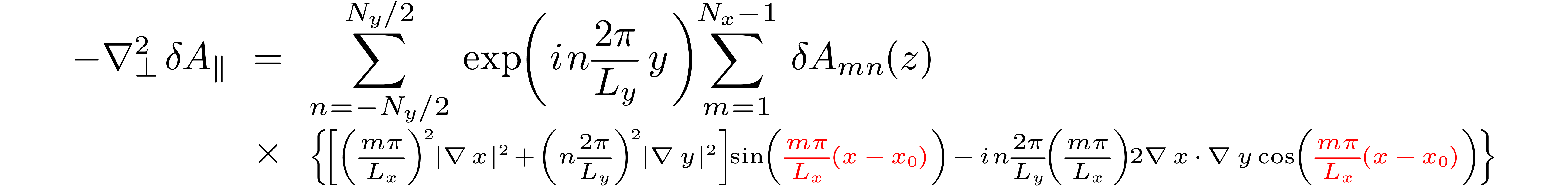
4.6Discretizing Laplacian operator
In TEK, the Laplacian operator is approximated as
 |
(205) |
which is called “high-n approximation”, in which all
derivatives with respect to  are dropped. This
approximation reduces the Laplacian differential operator from 3D to 2D.
are dropped. This
approximation reduces the Laplacian differential operator from 3D to 2D.
We assume that satisfies the zero boundary
condition in the  direction:
  . Then the sine expansion can be used in this
direction. In the
. Then the sine expansion can be used in this
direction. In the  direction, full Fourier
expansion is needed. I.e., at each value of ,
direction, full Fourier
expansion is needed. I.e., at each value of ,  is approximated by the
following two-dimensional expansion:
is approximated by the
following two-dimensional expansion:
 |
(206) |
Use this expression, then  of Eq. (205)
is written as
of Eq. (205)
is written as
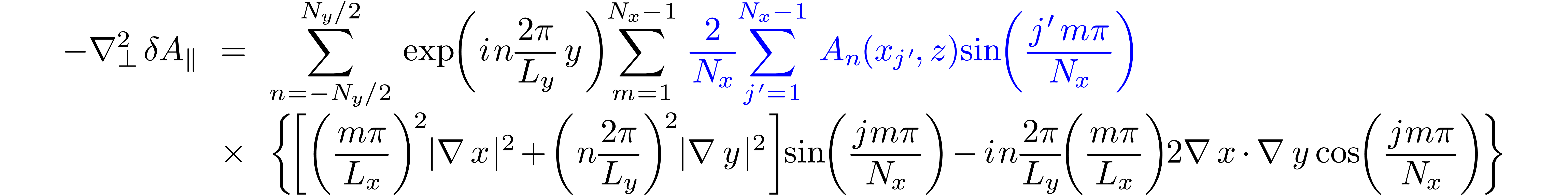
At  , with
  and
and  , the above expression is
written as
, the above expression is
written as
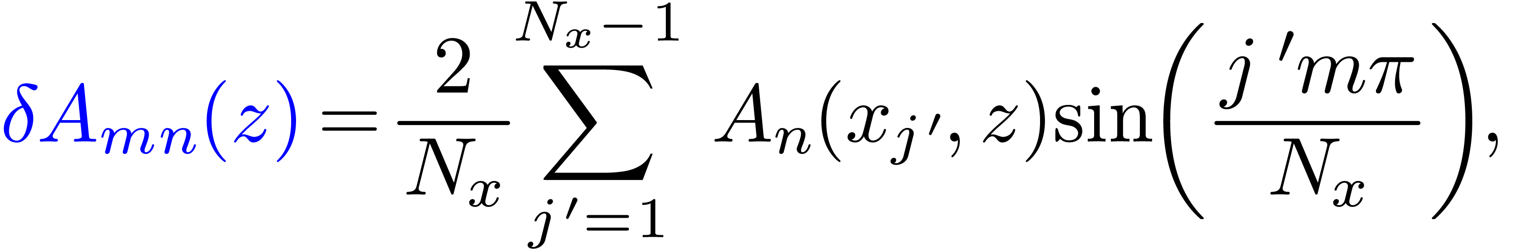
where and are evaluated
at  . Plugging the DST
coefficients
. Plugging the DST
coefficients
 |
(208) |
into expression (207) gives
For a single toroidal harmonic, the above expression reduces to
Define
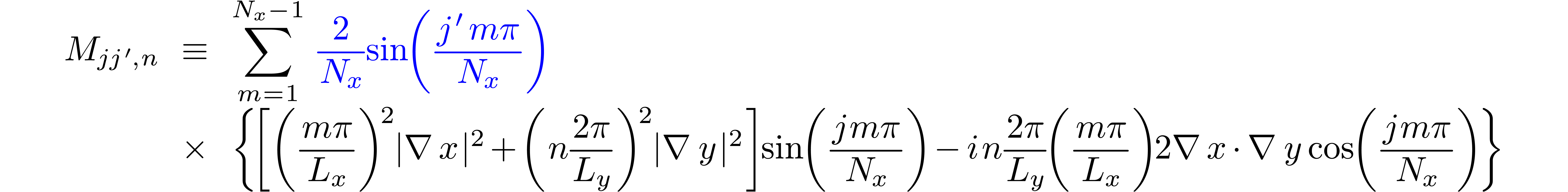
then expression (209) is written as
 |
(210) |
4.7Parallel Ampere's Law in GEM
code
 |
(211) |
where the parallel currents are given by
 |
(212) |
 |
(213) |
where  and
and  is the
parallel current carried by the distribution function , which are updated from the value at the
is the
parallel current carried by the distribution function , which are updated from the value at the  time step using an explicit scheme and therefore does
not depends on the field at the
time step using an explicit scheme and therefore does
not depends on the field at the  step. The blue terms in Eqs. (212) and (213)
are the “skin current”, which explicitly depend on the
unknown field at the step. If we want to solve
Ampere's law (211) by direct methods, then the blude terms
need to be moved to the left-hand side. In this case, equation (211)
is written as
step. The blue terms in Eqs. (212) and (213)
are the “skin current”, which explicitly depend on the
unknown field at the step. If we want to solve
Ampere's law (211) by direct methods, then the blude terms
need to be moved to the left-hand side. In this case, equation (211)
is written as
Then we need to put the blue terms into matrix form.
If we put the bule terms into martrix form by using numerical grid
integration (as we do for the polarization density), then there arises
the cancellation propblem (i.e., the two parts of the distribution are
evaluated by different methods, one is grid-based and the other is MC
marker based, there is a risk that the sum of the two terms will be
inaccurate when the two terms are of opposite signs and large
amplitudes, and the final result amplitude is expected to be much
smaller than the amplituded of the two terms). If we get the matrix form
by evaluating it numerically using MC markers (which can avoid the
cancellation problem), the corresponding matrix will depends on markers
and thus needs to be re-constructed each time-step, which is
computationally expensive.
Therefore we go back to Eq. (211) and try to solve it using
iterative methods. However, it is found numerically that directly using
Eq. (211) as an iterative scheme is usually divergent. To
obtain a convergent iterative scheme, we need to have an approximate
form for the blue terms (bigger terms), which is independent of markers
and so that it is easy to construct its matrix, and then subtract this
approximate form from both sides. After doing this, the iterative scheme
has better chance to be convergent (partially due to that the right-hand
side becomes smaller). An approximate form is that derived by neglecting
the FLR effect given in Sec. 4.4. Using this, the iterative
scheme for solving Eq. (211) is written as
In the drift-kinetic limit (i.e., neglecting the FLR effect), the blue
and red terms on the right-hand side of the above equation cancel each
other exactly. Even in this case, it is found numerically that these
terms need to be retained and the blue terms are evaluated using
markers. Otherwise, numerical inaccuracy can give numerical
instabilities, which is the so-called cancellation problem. The
explanation for this is as follows. The blue terms are part of the
current. The remained part of the current carried by  is computed by using Monte-Carlo integration over markers. If the blue
terms are evaluated analytically, rather than using Monte-Carlo
integration over markers, then the cancellation between this analytical
part and Monte-Carlo part can have large error (assume that there are
two large contribution that have opposite signs in the two parts)
because the two parts are evaluated using different methods and thus
have different accuracy, which makes the cancellation less accurate.
is computed by using Monte-Carlo integration over markers. If the blue
terms are evaluated analytically, rather than using Monte-Carlo
integration over markers, then the cancellation between this analytical
part and Monte-Carlo part can have large error (assume that there are
two large contribution that have opposite signs in the two parts)
because the two parts are evaluated using different methods and thus
have different accuracy, which makes the cancellation less accurate.
Because the ion skin current is smaller than its electron counterpart by
a factor of  , its accuracy is
not important. The cancellation error for ions is not a problem and
hence can be neglected. In this case, equation (215) is
simplified as
, its accuracy is
not important. The cancellation error for ions is not a problem and
hence can be neglected. In this case, equation (215) is
simplified as
Note that the blue term will be evaluated using Monte-Carlo markers.
4.8Split-weight scheme for electrons in GEM
code
The perturbed distribution function is decomposed as given by Eq. (157), i.e.,
 |
(217) |
where the term in blue is the so-called adiabatic
response, which depends on the gyro-angle in guiding-center coordinates.
Recall that the red term  ,
which is independent of the gyro-angle, is introduced in order to
eliminate the time derivative
,
which is independent of the gyro-angle, is introduced in order to
eliminate the time derivative  term on the
right-hand side of the original Frieman-Chen gyrokinetic equation.
term on the
right-hand side of the original Frieman-Chen gyrokinetic equation.
The so-called generalized split-weight scheme corresponds to going back
to the original Frieman-Chen gyrokinetic equation by introducing another
 term with a free small parameter
  . Specifically, in the
above is split as
. Specifically, in the
above is split as
 |
(218) |
(If  , then the two terms in Eq. (217) and (218)
cancel each other.) Substituting this expression into Eq. (), we obtain
the following equation for
, then the two terms in Eq. (217) and (218)
cancel each other.) Substituting this expression into Eq. (), we obtain
the following equation for  :
:
Noting that , ,  ,
we find that the third line of the above equation is
of order and thus can be dropped. Moving the second line to the right-hand side, the above equation
is written as
,
we find that the third line of the above equation is
of order and thus can be dropped. Moving the second line to the right-hand side, the above equation
is written as
4.8.1special case of 
For the special case of (the default and most
used case in GEM code, Yang Chen said  cases are sometimes not accurate, so he gave up using it since 2009),
equation (220) can be simplified as:
cases are sometimes not accurate, so he gave up using it since 2009),
equation (220) can be simplified as:
where two  terms cancel each other. Because the
 term is one of the factors that make kinetic
electron simulations difficult, eliminating term
may be beneficial for obtaining stable algorithms.
term is one of the factors that make kinetic
electron simulations difficult, eliminating term
may be beneficial for obtaining stable algorithms.
For ,
is written as
where the adiabatic term will be moved to the left-hand side of the
Poisson's equation. The descretization of this term is much easier than
the polarization density.
Equation (221) actually goes back to the original
Frieman-Chen equation. The only difference is that  is split from the perturbed distribution function. Considering this,
equation (221) can also be obtained from the original
Frieman-Chen equation (135) by writing
as
is split from the perturbed distribution function. Considering this,
equation (221) can also be obtained from the original
Frieman-Chen equation (135) by writing
as
 |
(223) |
In this case, is written as
 |
(224) |
Substituting expression (223) into equation (135),
we obtain the following equation for :
Noting that , , ,
we find that the third line of the above equation is of order and thus can be dropped. Moving the second line to the
right-hand side, the above equation is written as
which agrees with Eq. (221).
In GEM, the split weight method is used only for electrons. When using
this scheme,  appears on the right-hand-side of
the weight evolution equation. GEM makes use of the vorticity equation
(time derivative of the Poissson equation) to evaluate .
appears on the right-hand-side of
the weight evolution equation. GEM makes use of the vorticity equation
(time derivative of the Poissson equation) to evaluate .
5Poisson's equation and
polarization density
Poisson's equation for the potential perturbation
is written as
 |
(227) |
where  is the space-charge term (Debye shielding
term). Since we consider modes with
is the space-charge term (Debye shielding
term). Since we consider modes with  ,
the space-charge term is approximated as
,
the space-charge term is approximated as  .
Then Eq. (227) is written as
.
Then Eq. (227) is written as
 |
(228) |
This approximation eliminates the parallel plasma oscillation from the
system. The perpendicular plasma oscillations seem to be only partially
eliminated in the system consisting of gyrokinetic ions and
drift-kinetic electrons. There are the so-called
modes (also called electrostatic shear Alfven wave) that appear in the
gyrokinetic system which have some similarity with the plasma
oscillations but with a much smaller frequency,  .
.
Using expression (157), the density perturbation  is written as
where the blue term is approximately zero for
isotropic and this term is usually dropped in
simulations that assume isotropic and
approximate as  .
The red term in expression (229) is the
so-called the polarization density
.
The red term in expression (229) is the
so-called the polarization density  ,
i.e.,
,
i.e.,
 |
(230) |
which has an explicit dependence on and is
usually moved to the left hand of Poisson's equation when constructing a
numerical solver for the Poisson equation, i.e., equation (228)
is written as
 |
(231) |
where  , which is evaluated by
using Monte-Carlo markers. Since some parts depending on are moved from the right-hand side to the left-hand side
of the field equation, numerical solvers (for ) based on the left-hand side of Eq. (231)
may behave better than the one that is based on the left-hand side of
Eq. (228), i.e.,
, which is evaluated by
using Monte-Carlo markers. Since some parts depending on are moved from the right-hand side to the left-hand side
of the field equation, numerical solvers (for ) based on the left-hand side of Eq. (231)
may behave better than the one that is based on the left-hand side of
Eq. (228), i.e.,  .
.
5.1Discussion on cancellation scheme
We note that the polarization density  is part of
the density perturbation. is extracted from the
source term and moved to the left-hand side of the Poisson equation.
This term will be evaluated without using Monte-Carlo markers, whereas
the remained density on the right-hand side will be evaluated using
Mote-Carlo markers. The two different methods of evaluating two parts of
the density perturbation can possibly introduce significant errors if
the two terms are expected to cancel each other and give a small
quantity that is much smaller than either of the two terms. This is one
pitfall for PIC simulations that extract some parts from the source term
and move them to the left-hand side. To remedy this, rather than
directly moving a part of the distribution function to the left-hand
side, we subtract an (approximate) analytic expression from both sides
of Eq. (228). The analytical expressions on both sides are
evaluated based on grid values of perturbed electromagnetic fields and
are independent of makers. All the original parts of the distribution
functions are kept on the right-hand side and are still evaluated by
using markers, which hopefully avoids the possible cancellation problem.
This strategy is often called a cancellation scheme. Since unknown
perturbed electromagnetic fields appear on the right-hand side,
iteration is needed to solve the field equation.
is part of
the density perturbation. is extracted from the
source term and moved to the left-hand side of the Poisson equation.
This term will be evaluated without using Monte-Carlo markers, whereas
the remained density on the right-hand side will be evaluated using
Mote-Carlo markers. The two different methods of evaluating two parts of
the density perturbation can possibly introduce significant errors if
the two terms are expected to cancel each other and give a small
quantity that is much smaller than either of the two terms. This is one
pitfall for PIC simulations that extract some parts from the source term
and move them to the left-hand side. To remedy this, rather than
directly moving a part of the distribution function to the left-hand
side, we subtract an (approximate) analytic expression from both sides
of Eq. (228). The analytical expressions on both sides are
evaluated based on grid values of perturbed electromagnetic fields and
are independent of makers. All the original parts of the distribution
functions are kept on the right-hand side and are still evaluated by
using markers, which hopefully avoids the possible cancellation problem.
This strategy is often called a cancellation scheme. Since unknown
perturbed electromagnetic fields appear on the right-hand side,
iteration is needed to solve the field equation.
Note that two things appear here: What motivates us to move parts of the
distribution function to the left? It is the goal of hopefully making
the left-hand side matrix more well-behaved (such as good condition
number, etc.) Why do we need the cancellation scheme? Because we want to
avoid the numerical inaccuracy that appears when large terms cancels
each other. Note that iteration is needed when the cancellation scheme
is used because the right-hand side explicitly contains unknown
electromagnetic fields.
It turns out that the cancellation scheme is not necessary for the
Poisson Eq. (231), but for the field solver for Ampere's
equation (discussed later), this kind of cancellation scheme can be
necessary, e.g., in GEM's split weight method. For the mix-variable
pullback method, I found that the cancellation scheme is not necessary
even for Ampere's law (KBM results obtained with it and without it agree
with each other in the DIII-D cyclone base case).
6Polarization density matrix
We need to perform the gyro-average and velocity integration in the
polarization density (expression (230)) to obtain a matrix
form that relates the polarization density at gridpoints to at gridpoints, so that the corresponding matrix form of
the left-hand side of Poisson's equation (231) can be
inverted to solve for .
The dependence of the first term in expression (230) (often
called adiabatic term) on is trivial (because
is independent of the velocity in particle
coordinates):
If we assume is Maxwellian, then the velocity
integration can be analytically performed:
Next, let us consider the more complicated term, the second term in
expression (230), i.e.,
 |
(234) |
At particle location , we
construct local (velocity) cylindrical coordinates  . Then the velocity element is given by
  . Then the above integration is
written as
. Then the above integration is
written as
 |
(235) |
Note that  (in terms of particle coordinates)
dpends on . But this
dependence is usually weak and neglected. So it is moved outside of the
integration. Note that the above is a velcoity
space integration for a fixed particle position.
(in terms of particle coordinates)
dpends on . But this
dependence is usually weak and neglected. So it is moved outside of the
integration. Note that the above is a velcoity
space integration for a fixed particle position.
Using the definition of the gyro-averaging  ,
expression (235) is written as
,
expression (235) is written as
 |
(236) |
Here the gyro-averaging can be understood as time integration of the
gyro-orbit that has the point on its trajectory.
The gyro-phase when the particle is passing is
. So its guiding-center
location can be calculated as
 |
(237) |
Using , the full gyro-ring is
written as (parameterized by )

i.e.,
 |
(238) |
Then expression (236) is written as
To proceed, we have two options. One is to assume no analytical
expression of  and use pure numerical
interpolation to handle the above integration, and finally expression it
as combination of values on gridpoints. Another
option is to assume basis function expansion of
and perform analytically the integration for each basis function. The
first option is further discussed in Sec. 6.2. Next, we
focus on the second option and use Fourier expansion.
and use pure numerical
interpolation to handle the above integration, and finally expression it
as combination of values on gridpoints. Another
option is to assume basis function expansion of
and perform analytically the integration for each basis function. The
first option is further discussed in Sec. 6.2. Next, we
focus on the second option and use Fourier expansion.
6.1In terms of Fourier basis functions
We Fourier expand as
 |
(240) |
where  is the expansion coefficients. Then
expression (239) is written as
is the expansion coefficients. Then
expression (239) is written as
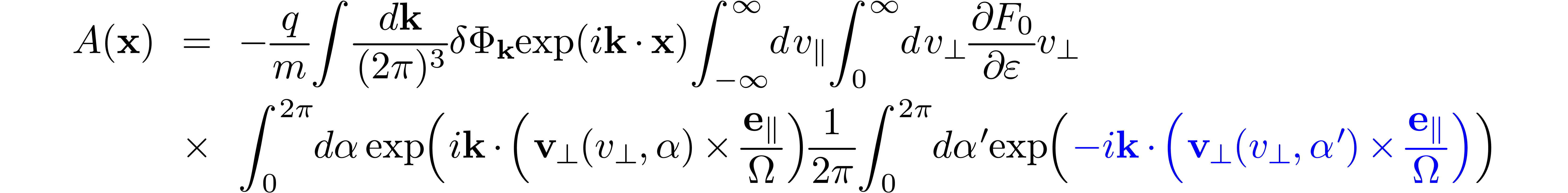
Let  define one of the perpendicular direction
 , i.e.,
  . Then another perpendicular basis vector is
defined by
. Then another perpendicular basis vector is
defined by  . Then is written as
  ,
which defines the gyro-angle .
Then the blue term is written as
,
which defines the gyro-angle .
Then the blue term is written as
Then the integration is written as
where use has been made of the definition of the zeroth Bessel function
of the first kind.
Similarly, the integration is also reduced to
 . Then
  is written as
 |
(243) |
6.1.1The remaining velocity integration can be
performed analytically if is Maxwellian
If is a Maxwellian distribution, then the
remaining velocity integration in Eq. (243)can be
analytically performed. Maxwelliand distribution is given by
where  , then
 |
(246) |
As is mentioned above, we ignore the weak dependence of  and
and  on (introduced by
 ) when transformed back to
particle coordinates. (For sufficiently large velocity, the
corresponding Larmor radius will be large enough to make the equilibrium
undergo substantial variation. Since the velocity integration limit is
to infinite, this will definitely occur. However,
is exponentially decreasing with velocity, making those particles with
velocity much larger than the thermal velocity negligibly few and thus
can be neglected.)
) when transformed back to
particle coordinates. (For sufficiently large velocity, the
corresponding Larmor radius will be large enough to make the equilibrium
undergo substantial variation. Since the velocity integration limit is
to infinite, this will definitely occur. However,
is exponentially decreasing with velocity, making those particles with
velocity much larger than the thermal velocity negligibly few and thus
can be neglected.)
Parallel integration
Using Eq. (246), the expression in the square brackets of
Eq. (243) is written as
where  ,
,  . Using
 |
(249) |
the integration over  in expression (248)
can be performed, yielding
in expression (248)
can be performed, yielding
 |
(250) |
Perpendicular integration
Using (I verified this by using Sympy)
 |
(251) |
where  is the zeroth modified Bessel function of
the first kind, expression (250) is written
is the zeroth modified Bessel function of
the first kind, expression (250) is written
 |
(252) |
where  . Then the
corresponding density (234) is written as
. Then the
corresponding density (234) is written as
 |
(253) |
In Fourier space, the adiabatic term in expression (233) is
written as
 |
(254) |
Plugging expression (253) and (254) into
expression (230), the polarization density
is written as
 |
(255) |
Define
 |
(256) |
then Eq. (255) is written as
 |
(257) |
Expression (257) agrees with the result given in Yang
Chen's notes. Note that the dependence on species mass enters the
formula through the Larmor radius  in
in  .
.
6.1.2Pade approximation
defined in Eq. (256) can be
approximated by the Pade approximation as
 |
(258) |
The comparison between the exact value of and
the above Pade approximation is shown in Fig. 1.
Using the Pade approximation (258), the polarization
density in expression (257) can be
written as
 |
(259) |
6.1.3Long wavelength approximation of the
polarization density
In the long wavelength limit,  ,
expression (259) can be further approximated as
,
expression (259) can be further approximated as
Then the corresponding term in the Poisson equation is written as
where  is the Debye length defined by
  . For typical tokamak plasmas, the
thermal ion gyroradius is much larger than . Therefore the term in expression
(261) for ions is much larger than the space charge term
in the Poisson equation. Therefore the space
charge term can be neglected in the long wavelength limit.
. For typical tokamak plasmas, the
thermal ion gyroradius is much larger than . Therefore the term in expression
(261) for ions is much larger than the space charge term
in the Poisson equation. Therefore the space
charge term can be neglected in the long wavelength limit.
Equation (261) also shows that electron polarization
density is smaller than the ion polarization density by a factor of
 . Note that this conclusion
is drawn in the long wavelength limit. For short wavelength, the
electron polarization and ion polarization density can be of similar
magnitude (to be discussed later).
. Note that this conclusion
is drawn in the long wavelength limit. For short wavelength, the
electron polarization and ion polarization density can be of similar
magnitude (to be discussed later).
6.1.4Polarization density expressed in terms
of Laplacian operator
The polarization density expression (260) is for the long
wavelength limit, which partially neglects FLR effect. Let us go back to
the more general expression (259). The Poisson equation is
written
 |
(262) |
Write  , where
  is the ion polarization density, then the above expression
is written
is the ion polarization density, then the above expression
is written
 |
(263) |
Fourier transforming in space, the above equation is written
 |
(264) |
where  is the Fourier transformation (in space)
of the polarization density
is the Fourier transformation (in space)
of the polarization density  and similar meanings
for
and similar meanings
for  ,
,  , and
, and  .
Expression (259) implies that is
given by
.
Expression (259) implies that is
given by
 |
(265) |
Using this, equation (264) is written
 |
(266) |
Multiplying both sides by  ,
the above equation is written
,
the above equation is written
 |
(267) |
Next, transforming the above equation back to the real space, we obtain
 |
(268) |
Neglecting the Debye shielding term, the above equation is written
 |
(269) |
which is the equation actually solved in many gyrokinetic codes, where
 .
.
6.2Polarization density obtained by
numerical integration
In Sec. 6, to evaluate the polarization density, the
potential is Fourier expanded in space, and then
the double gyro-angle integration of each harmonic is expressed as the
Bessel function. (This method is often used in numerical codes that use
specrum expansion in both radial and toroidal direction, where the local
perpendicular wave number can be easily calculated numerically. The GEM
code uses this method.) In this section, we avoid using the local
Fourier expansion, and directly express the double gyro-angle integral
as linear combination of values of at spatial
grid-points.
6.3Direct evaluation of the double gyrophase
integration
Then is written as
where  is the number of points chosen for discretization,
  is the number
of points chosen for discretization. For
notation ease, define
is the number
of points chosen for discretization. For
notation ease, define
 |
(271) |
which is a function of  . Then
Eq. (270) is written as
. Then
Eq. (270) is written as
 |
(272) |
The guiding-center transform and its inverse used in the above are
illustrated in Fig. 2.
Let us summarize the above algorithm. Given  , the double gyro-angle integration at a particle
location
, the double gyro-angle integration at a particle
location  is evaluated by the following steps:
The above 3 steps specify how to approximate the double gyro-angle
integration as the sum of values of at discrete
spatial points  . The spatial
points are not necessarily grid points.
Interpolations are used to further express
. The spatial
points are not necessarily grid points.
Interpolations are used to further express  as
weighted combination of values at gridpoints.
as
weighted combination of values at gridpoints.
6.4Toroidal DFT of polarization density in
field-aligned coordinates
In the field-aligned coordinates ,
Fourier expand along :
 |
(274) |
where  ,
,  is an even integer specifying how many harmonics are included,
  is the expansion coefficient. Using expression (274)
in Eq. (272), we obtain
is the expansion coefficient. Using expression (274)
in Eq. (272), we obtain
From Eq. (275), the Fourier expansion coefficient of  can be identified:
Assume each toroidal harmonic amplitude  is
weakly varying along field line, then we can make the following
approximation:
is
weakly varying along field line, then we can make the following
approximation:
 |
(277) |
because the variation along a field line over a distance of a Larmor
radius is small. Then expression (276) is written as
The approximation (277) makes the dependence of  on become local in the direction, i.e., at
  only involves values of at . Meanwhile
at
only involves values of at . Meanwhile
at  involves values of at
 besides .
6.4.1For Maxwelliand distribution
Assume that is Maxwellian, then
 |
(279) |
Note that  is independent of . Then the integration over
in Eq. (278) can be analytically performed:
is independent of . Then the integration over
in Eq. (278) can be analytically performed:

where  , and use has been made
of
, and use has been made
of
 |
(280) |
6.4.2Using sine expansion for the radial
dependence of
Expand in terms of sine basis functions  :
:
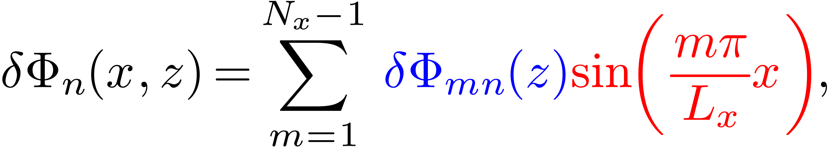 |
(281) |
i.e.,
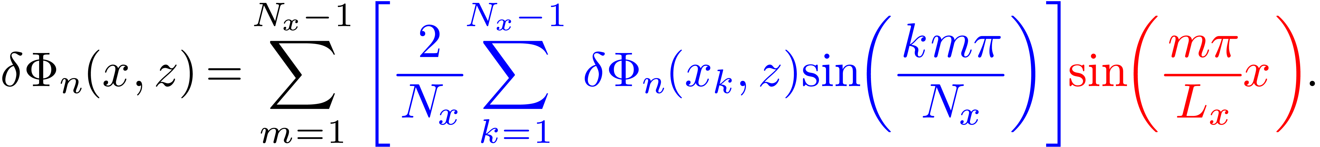 |
(282) |
For a given  and at a given , consider
  with
with  as a column vector, and similarly
  with
with  as a column vector. Then the two column
vectors are related by the following matrix form:
as a column vector. Then the two column
vectors are related by the following matrix form:

where  is a
is a  matrix with
its elements given by
matrix with
its elements given by

7TEK benchmarking with GENE in DIII-D cyclone
base case
The DIII-D cyclone base case is a circular and concentric magnetic
configuration. The main parameters are summarized in Table 1.
All parameters are the same as those in T. Gorler's paper[4].
(This configuratgion was inspired by DIII-D H-mode discharge #81499 and
used in the cyclone project for benchmarking various gyrokinetic ITG
turbulence simulations.)
The safety factor profile is chosen as [6]

This profile gives  and
and  at
at  . The equilibrium ion
temperature and number density profile are given by
. The equilibrium ion
temperature and number density profile are given by
 |
(283) |
 |
(284) |
where  ,
,  ,
,  .
Then the radial derivatives are written as
.
Then the radial derivatives are written as

The corresponding gradient scale lengths of  and
and
 are then given by
 |
(285) |
and
 |
(286) |
where  . The electron density
and temperature profiles are assumed to be identical to those of ions.
The electron mass is set as
. The electron density
and temperature profiles are assumed to be identical to those of ions.
The electron mass is set as  ,
i.e., two times the realistic value of electron mass.
,
i.e., two times the realistic value of electron mass.
The profiles of safety factor, temperature, and density are plotted in
Fig. 3.
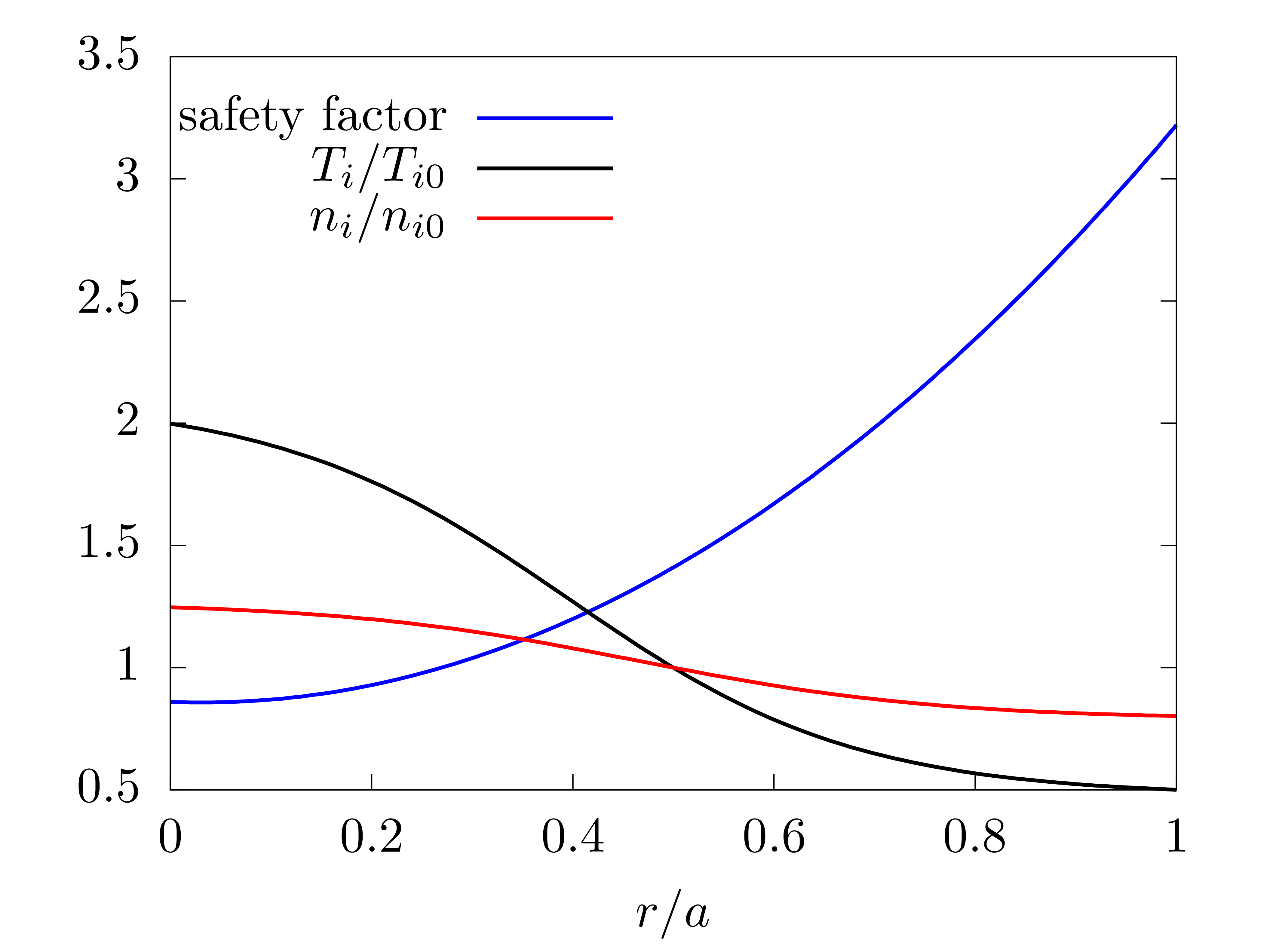 |
|
Figure 3. Radial profiles of safety
factor, temperature, and density of the above DIII-D cyclone
test case. The dashed lines indicate the radial simulation box
 . .
|
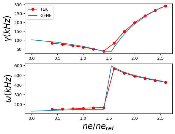
|
|
Figure 4. Benchmarking of TEK code with GENE
for the ITG-KBM transition. Upper panel: growth rate; lower
panel: angular frequency.
|
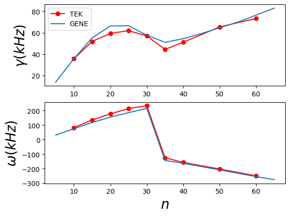
|
|
Figure 5. ITG-TEM transition benchmarking
|
Mode structures:
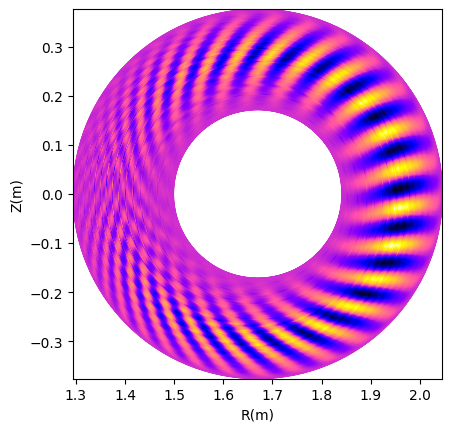 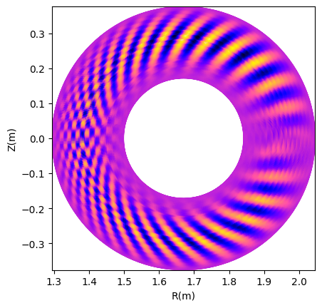
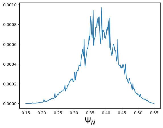 1.6022d-16 1.6022d-16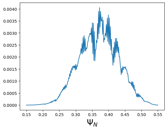
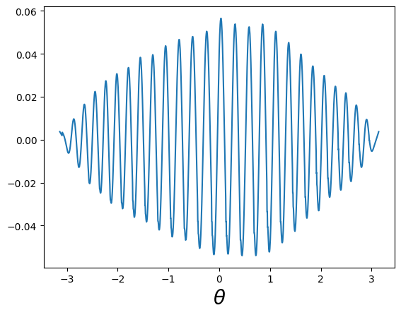 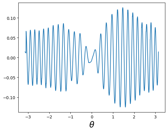
|
|
Figure 6. ITG  . .
|
ITG-KBM transition:
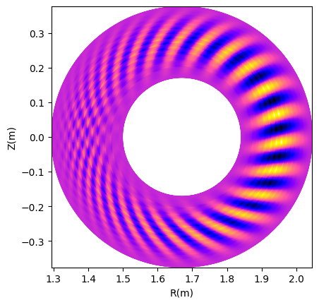 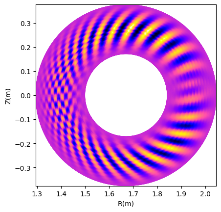
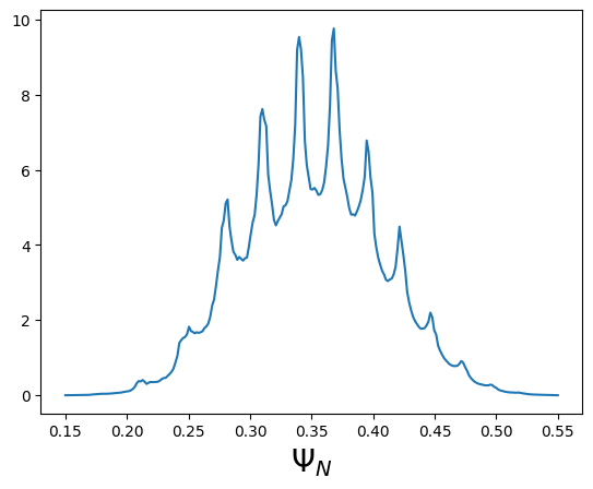 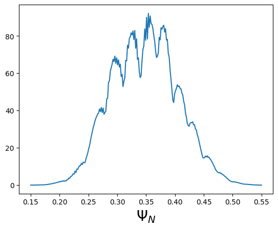
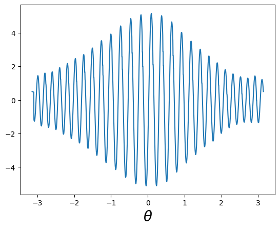 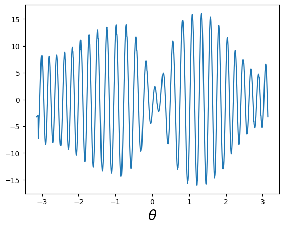
|
|
Figure 10. The same as Fig. 9
excep the radial range is narrowed.
|
8Heat diffusivity
A general conservation law for a scalar quantity  can be written as
 |
(287) |
where  is a source term, and
  is the flux, which can often be divided into two terms: the diffusive
term and convective term, i.e.,
is the flux, which can often be divided into two terms: the diffusive
term and convective term, i.e.,
 |
(288) |
where  is called the diffusivity,
  is the flow velocity that transports .
[If  and is constant,
then Eq. (287) without the source term reduces to the
following parabolic equation:
and is constant,
then Eq. (287) without the source term reduces to the
following parabolic equation:
 |
(289) |
which is often called diffusion equation.]
Next, let us neglect the convection, i.e., set . For the case of energy diffusion,
is the kinetic energy density, i.e.,  ,
where
,
where  is the number density and
  is the temperature. Assuming that is constant in
space, then the diffusivity in Eq. (288)
can be written as
is the temperature. Assuming that is constant in
space, then the diffusivity in Eq. (288)
can be written as
 |
(290) |
In studying tokamak energy transport, it is the radial component that is
of interest. The energy radial diffusivity (or conductivity) is defined as
 |
(291) |
where is the flux-surface average, and  is the radial energy flux defined by
 |
(292) |
where  ,
,  is the equilibrium drift,
  is the drift
perturbation, is the distribution function
perturbation. The flux contributed by the equilibrium drift (i.e.,
linear flux) is usually small and neglected [The equilibrium drift has
only
is the drift
perturbation, is the distribution function
perturbation. The flux contributed by the equilibrium drift (i.e.,
linear flux) is usually small and neglected [The equilibrium drift has
only  component. The fulx-surface averaging will
make all the
component. The fulx-surface averaging will
make all the  components
multiplied by the equilibrium be zero. Only
component (zonal component) of ,
multiplied by the equilibrium drift can give nonzero flux. For this flux
to be significant, the zonal component usually needs to be very strong.]
components
multiplied by the equilibrium be zero. Only
component (zonal component) of ,
multiplied by the equilibrium drift can give nonzero flux. For this flux
to be significant, the zonal component usually needs to be very strong.]
The perturbed distribution function contains a term:  , i.e., the polarization term. This term's
contribution to the heat flux is usually small and is ignored (confirmed
by Ye Lei).
, i.e., the polarization term. This term's
contribution to the heat flux is usually small and is ignored (confirmed
by Ye Lei).
Equation (291) indicates that the unit of
in SI units is  .
.
8.0.1Bohm and gyroBohm scaling
For a species  , the gyro-Bohm
energy diffusivity is defined by
, the gyro-Bohm
energy diffusivity is defined by
 |
(293) |
whereas the Bohm diffusivity is defined by
 |
(294) |
where is the species label,  is the thermal speed,
  is the thermal Larmor
radius,
is the thermal Larmor
radius,  is the cyclotron frequency,
  is the radial gradient scale length of temperature or
density of species . Because
evolves in gyrokinetic
simulations without source terms, some autors prefer to replace in the above definition by the minor radius of the
LCFS,
is the radial gradient scale length of temperature or
density of species . Because
evolves in gyrokinetic
simulations without source terms, some autors prefer to replace in the above definition by the minor radius of the
LCFS,  .
.
Comparing Eqs. (293) and (294), we know that
the Bohm diffusivity is  times larger than the
gyroBohm one. The energy diffusitivity observed in gyrokinetic
simulations usuall is much samller than
times larger than the
gyroBohm one. The energy diffusitivity observed in gyrokinetic
simulations usuall is much samller than  and is
often of the same order of
and is
often of the same order of  .
.
The Bohm diffusitivity can also be written as:
 |
(295) |
which is independent of the machine size, and the gyro-Bohm
diffusitivity can be written as
 |
(296) |
where is replaced by the minor radius of the
LCFS, . The gyro-Bohm
diffusitivity decreases with increasing machine size. The gyro-Bohm
diffusivity is proportional to  ,
which means heavier isotops have larger diffusivity if the satisfy the
gyro-Bohm scaling.
,
which means heavier isotops have larger diffusivity if the satisfy the
gyro-Bohm scaling.
AAdiabatic electron response
Assume that the total electron density satisfies the Boltzmann
distribution on each magnetic surface, i.e.,
 |
(297) |
where  is a radial function. Note that this does
not imply that the equilibrium density is (it
just implies that the total density is at the
location where
is a radial function. Note that this does
not imply that the equilibrium density is (it
just implies that the total density is at the
location where  , which can
still be different from the equilibrium density).
, which can
still be different from the equilibrium density).
Further assume that the magnetic surface average of electron density
perturbation ( ) is zero,
i.e.,
) is zero,
i.e.,
 |
(298) |
where  is the equilibrium electron density,
  is the magntic surface averaging operator. Using Eq.
(297) in the above condition, we get
is the magntic surface averaging operator. Using Eq.
(297) in the above condition, we get
 |
(299) |
Then expression (297) is written as
 |
(300) |
Then the perturbation is written as
 |
(301) |
This model for electron response is often called adiabatic electron.
A.1Poisson's equation with adiabatic electron
response
Pluging expression (301) into the Poisson equation (231), we get
 |
(302) |
When solving the Poisson equation, the equation is Fourier expanded into
toroidal harmonics. Each harmonic is independent of each other, so that
they can be solved independently. For harmonics,
the  terms is zero and thus the the electron term
is easy to handle because it's a local response. There is some
difficulty in solving the harmonic because the
terms is zero and thus the the electron term
is easy to handle because it's a local response. There is some
difficulty in solving the harmonic because the
 term is nonzero.
I use the following method to obtain .
First slove the harmonic of the following
equation:
 |
(303) |
(i.e., Eq. (302) with the electron contribution dropped).
Let  denote the solution to this equation. Then
it can be proved that
denote the solution to this equation. Then
it can be proved that  is equal to . [Proof:
Taking the flux surface average of Eq. (302), we obtain
 |
(304) |
where the adiabatic response disappears. to be continued.
]
Then solving Eq. (302) becomes easier because term is known and can be moved to the right-hand side as a
source term.
BCharacteristic curves of Frieman-Chen
gyrokinetic equation
Examining the left-hand side of Eq. (), the characteristic curves of
this equation can be identified:
 |
(305) |
 |
(306) |
 |
(307) |
(Note that the kinetic energy is conserved along
the characteristic curves while the real kinetic energy of a particle is
usually not conserved in a perturbed electromagnetic field. This may be
an indication that Frieman-Chen equation neglects the velocity space
nonlinearity.) For notation ease, we denote the total guiding-center
velocity by  , i.e.,
 |
(308) |
where
 |
(309) |
In the above, can be obtained by using  . However
is not easy to determine since it changes with time for trapped
particles. In practice, we get from an evolution
equation, which can be obtained by combining the equations for and . Next, we
derive this equation.
. However
is not easy to determine since it changes with time for trapped
particles. In practice, we get from an evolution
equation, which can be obtained by combining the equations for and . Next, we
derive this equation.
B.1Time evolution equation for 
Using the definition  ,
equation (307), i.e.,
,
equation (307), i.e.,  ,
is written as
,
is written as
 |
(310) |
which is written as
 |
(311) |
which can be further written as
 |
(312) |
Using the definition of the characteristics, the right-hand side of the
above equation can be expanded, giving
 |
(313) |
where  ,
,  , and
, and  are given by Eq.
(305), (306), and (307),
respectively. Using Eqs. (305)-(307) and
are given by Eq.
(305), (306), and (307),
respectively. Using Eqs. (305)-(307) and  , equation (313) is
reduced to
, equation (313) is
reduced to
 |
(314) |
On the other hand, equation (306), i.e.,  , is written as
 |
(315) |
which can be further written as
 |
(316) |
Using Eq. (314), the above equation is written as
 |
(317) |
which is the equation for the time evolution of . This equation involves , i,e., the guiding-center drift, which is given by
Eq. (305). Equation (317) for
can be simplified by noting that the Frieman-Chen equation is correct
only to the second order, ,
and thus the characteristics need to be correct only to the first order
and higher order terms can be dropped. Note
that, in the guiding-center drift given by Eq.
(305), only the  term in is of
order , all the other terms
are of . Using this, accurate
to order , equation (317)
is written as
term in is of
order , all the other terms
are of . Using this, accurate
to order , equation (317)
is written as
 |
(318) |
which is the time evolution equation ready to be used for numerically
advancing . Note that only
the mirror force  appears in Eq. (318)
and there is no parallel acceleration term
appears in Eq. (318)
and there is no parallel acceleration term  in
Eq. (318). This is because
in
Eq. (318). This is because  is of
order and (**check** the terms involving
is of
order and (**check** the terms involving  are of or higher and thus
have been dropped in deriving Frieman-Chen equation.)
are of or higher and thus
have been dropped in deriving Frieman-Chen equation.)
CFrom  to
to 
C.1Expression of  in
terms of
in
terms of 
Note that
Correct to order ,  in the above equation is written as (
vector can be considered as constant because its spatial gradient
combined with will give terms of , which are neglected)
in the above equation is written as (
vector can be considered as constant because its spatial gradient
combined with will give terms of , which are neglected)
Using local cylindrical coordinates  with being along the local direction of , and two components of
  being
being  and
and  ,
then
,
then  is written as
 |
(322) |
Note that the parallel gradient operator  acting
on the the perturbed quantities will result in quantities of order . Retaining terms of order up to
, equation (322)
is written as
acting
on the the perturbed quantities will result in quantities of order . Retaining terms of order up to
, equation (322)
is written as
 |
(323) |
i.e., only the parallel component survive, which exactly cancels the
last term in Eq. (321), i.e., equation (321)
is reduced to
 |
(324) |
C.1.1Using basis vectors in field-aligned
coordinates
In terms of  and
and  ,
is written as
,
is written as
 |
(325) |
Dotting the above equation by and , respectively, we obtain
 |
(326) |
 |
(327) |
Equations (326) and (327) can be further
written as
 |
(328) |
and
 |
(329) |
The solution of this  system is expressed by
Cramer's rule in the code.
system is expressed by
Cramer's rule in the code.
Use 

C.2Expression of  in
terms of
in
terms of
Accurate to , in the above equation is written as (
vector can be considered as constant because its spatial gradient
combined with will give
terms, which are neglected)
[Using local cylindrical coordinates with being along the local direction of , and two components of  being
being  and
and  ,
then
,
then  is written as
 |
(332) |
Note that the parallel gradient operator acting
on the the perturbed quantities will result in quantities of order . Retaining terms of order up to
, equation (322)
is written as
|
(333) |
Using this, equation (331) is written as
 |
(334) |
However, this expression is not useful for GEM because GEM does not use
the local coordinates .]
C.3Expressing the
perturbed drift in terms of  and
and 
The perturbed drift is given by Eq. (138),
i.e.,
 |
(335) |
Using , the above expression
can be further written as
Accurate to order , the term
involving is
which is the drift. Accurate to , the  term on the
right-hand side of Eq. (336) is written
term on the
right-hand side of Eq. (336) is written
which is called “magnetic fluttering” (this is actually not
a real drift). In obtaining the last equality, use has been made of Eq.
(324), i.e.,  .
.
Accurate to , the last term
on the right-hand side of expression (336) is written

Using equation (331), i.e.,  ,
the above expression is written as
,
the above expression is written as
where use has been made of  (**seems wrong**),
where the error is of
(**seems wrong**),
where the error is of  . The
term
. The
term  is of and thus can
be neglected (I need to verify this).
is of and thus can
be neglected (I need to verify this).
Using Eqs. (337), (339), and (340),
expression (336) is finally written as
 |
(341) |
Using this, the first equation of the characteristics, equation (305), is written as
C.4Expressing the coefficient before
in terms of and
[Note that
 |
(344) |
where  is of .
This means that
is of .
This means that  is of
although both
is of
although both  and
and  are of
.]
are of
.]
Note that
where use has been made of  ,
This indicates that
,
This indicates that  is of
is of  . Using Eq. (345), the coefficient
before in Eq. (143) can be further
written as
. Using Eq. (345), the coefficient
before in Eq. (143) can be further
written as
Using Eq. (346) and (), gyrokinetic equation (143)
is finally written as
DCoordinate system and grid in TEK
code
In  coordinates:
In this convention, the Jacobian of the
coordinate system,  is negative, i.e., is a left-handed system. The field-line-following
coordinate system
is negative, i.e., is a left-handed system. The field-line-following
coordinate system  is also a left-handed system.
The coordinate system
is also a left-handed system.
The coordinate system  is a right-handed system.
D.1Poloidal grid
I do not need to make connection with GEM's equilibrium poloidal array
because there is no coupling of equilibrium quantities between the code
written by me and the original code in GEM. The coupling happens for the
perturbed quanties, whose poloidal grids need to be consistent.
-
The gridpoint number along for perturbations
is denoted by mpol2. Its value is not chosen by users.
Instead, it is equal to numproc/ntube, i.e., mpol2
is the total number of cells along for MPI
parallelation. (numproc and ntube must be chosen
in a way that makes numproc/ntube an integer.)
-
Poloidal grid-points for perturbations are indexed as
0:mpol2-1, with 0 corresponding to and mpol2 corresponding to  . Field equations are solved at
  . (The field at mpol2, i.e., , is not identical to that at
due to toroidal shift of a magnetic field
line when it finish one poloidal loop, and is obtained by toroidally
inerpolating the fields at .)
No array for this is actually used in the code. The indexes just
correspond to gclr of MPI processors.
. (The field at mpol2, i.e., , is not identical to that at
due to toroidal shift of a magnetic field
line when it finish one poloidal loop, and is obtained by toroidally
inerpolating the fields at .)
No array for this is actually used in the code. The indexes just
correspond to gclr of MPI processors.
-
The equilibrium poloidal gridpoint number, mpol, must be
chosen in a way that makes (mpol-1)/mpol2 an integer, which
can be larger than 1, i.e., one simulation cell can span several
equilibrium cells.
D.2Toroidal grid
D.3Radial grid
GEM array index system is better than TEK's because my system is not
consistent: sometimes I use 0-based index and sometimes I use 1-based
index, sometimes the index ends at n and sometimes ends at n+1. It is
important to know accurately the transformation between the two systems.
EImplementation of gyrokinetics in
particle-in-cell (PIC) codes
E.1Inverse guiding-center transform in
field-following coordinates (x,y,z)
Define two unit vectors:
 |
(348) |
 |
(349) |
both of which are perpendicular to the equilibrium magnetic field. Then
a random gyro-radius vector  can be constructed
by
can be constructed
by
 |
(350) |
where  is a random angle in
  among different markers, is an angle variable in
that will be discretized with uniform intervals
for each marker, and
among different markers, is an angle variable in
that will be discretized with uniform intervals
for each marker, and  is the gyro-radius
calculated using the magnetic field at the guiding-center location
is the gyro-radius
calculated using the magnetic field at the guiding-center location  . Then the particle location
  corresponding to this Larmor vector can be
approximated by the Talor expansion at :
corresponding to this Larmor vector can be
approximated by the Talor expansion at :
 |
(351) |
Using expressions (348), (349), (350),
equation (351) is written as
 |
(352) |
where , , and are all evaluated
at the guiding-center position .
E.2Monte-Carlo evaluation of distribution
function moment at grid-points
Suppose that the 6D guiding-center phase-space
is described by  coordinates, where is the gyro-angle. Denote the Jacobian of the coordinate
system by
coordinates, where is the gyro-angle. Denote the Jacobian of the coordinate
system by  .
.
Suppose that we sample the 6D phase-space by using a probability
function  . (Then the
effecitive probability function used in rejection method is
. (Then the
effecitive probability function used in rejection method is 
 .) Note that we
will sample a distribution function
.) Note that we
will sample a distribution function  that happens
to be independent of the gyro-angle .
Since
that happens
to be independent of the gyro-angle .
Since  is uniform in , it is natural to smaple
using a uniform probability function, i.e.,
is uniform in , it is natural to smaple
using a uniform probability function, i.e.,  can
be chosen to be independent of .
Then the weight is also independent of .
In terms of sampling , there
is no need to specify because both and marker distribution
can
be chosen to be independent of .
Then the weight is also independent of .
In terms of sampling , there
is no need to specify because both and marker distribution  are
indepedent of . However,
sampling is still necessary in simulations. From
the perspective of programming, it is ready to understand why needs to be specified: when computing density at
grid-points, we need to compute particle locations from the
guiding-center locations which requires us to specify the gyro-angle
for each marker. Specifically, markers in
guiding-center space
are
indepedent of . However,
sampling is still necessary in simulations. From
the perspective of programming, it is ready to understand why needs to be specified: when computing density at
grid-points, we need to compute particle locations from the
guiding-center locations which requires us to specify the gyro-angle
for each marker. Specifically, markers in
guiding-center space  with fixed
  but different values of correspond to markers in
particle space with different locations (and different ). In the PIC method of computing or
but different values of correspond to markers in
particle space with different locations (and different ). In the PIC method of computing or  at fixed , the contribution of each particle marker to the
density is affected by the distance of the particle marker to the fixed
. Therefore different values
of contributes differently to
or , and thus the resolution
of matters.
at fixed , the contribution of each particle marker to the
density is affected by the distance of the particle marker to the fixed
. Therefore different values
of contributes differently to
or , and thus the resolution
of matters.
For a marker with coordinators  ,
the corresponding particle position can be calculated by using the
inverse guiding-center transformation (29). Then we can
deposit the marker weight to grid-points in the same way that we do in
conventional PIC simulations. Looping over all markers, we build the
particle density at grids.
,
the corresponding particle position can be calculated by using the
inverse guiding-center transformation (29). Then we can
deposit the marker weight to grid-points in the same way that we do in
conventional PIC simulations. Looping over all markers, we build the
particle density at grids.
Compared with conventional PIC methods, where particle positions are
directly sampled, what is the benefit of sampling guiding-center
positions and then transform them back to the particle positions? More
computations are involved since we need to numerically perform the
inverse guiding-center transformation. The answer lies in the important
fact that the distribution function  that needs
to be numerically evaluated in gyrokinetic simulation is actually
independent of the gyro-angle .
Furthermore, we use a probability density function
that needs
to be numerically evaluated in gyrokinetic simulation is actually
independent of the gyro-angle .
Furthermore, we use a probability density function  that is independent of to sample the 6D phase
space . Then the marker
weight
that is independent of to sample the 6D phase
space . Then the marker
weight  is independent of , where
  is number of markers
loaded. This fact enable resolution in particle coordinates can be
increased in a trivial way, as described below.
is number of markers
loaded. This fact enable resolution in particle coordinates can be
increased in a trivial way, as described below.
Suppose we have a concrete sampling of in the 6D
phase-space , i.e.,  with
with  , then we
can do the inverse guiding-center transform and then deposit particles
to the grids to obtain a moment (e.g. density).
, then we
can do the inverse guiding-center transform and then deposit particles
to the grids to obtain a moment (e.g. density).
Since  is independent of , the sampli Maybe the real reason is that I lack
the interests in learning them.ng
is independent of , the sampli Maybe the real reason is that I lack
the interests in learning them.ng  with
with  are uniform distributed random numbers. Therefore we can
generate another sampling of (denoted by
are uniform distributed random numbers. Therefore we can
generate another sampling of (denoted by  with )
using random number generators and combine with
the old sampling
with )
using random number generators and combine with
the old sampling  to obtain a new sampling
  . The values of
  at the new sampling points are equal to the original values, i.e.,
  since the particle weight
  is
independent of . Using the
new sampling and following the same procedures given above, we can
estimate values of the moment at grid-points again, which will differ
from the estimation obtained using the old sampling because the
resulting sampling of and
for is different. Taking the average of the two
estimations will give a more accurate estimation because the resolution
in x and for is increased.
is
independent of . Using the
new sampling and following the same procedures given above, we can
estimate values of the moment at grid-points again, which will differ
from the estimation obtained using the old sampling because the
resulting sampling of and
for is different. Taking the average of the two
estimations will give a more accurate estimation because the resolution
in x and for is increased.
[Note that even if is dependent on due to the possible dependence of  on , we still can easily
generate a new set of sampling which differs from the old sampling only
in . Specifically, in the
rejection method, we use the old sampling for
each reject step and only adjust to satisfy the
acceptance criteria.]
on , we still can easily
generate a new set of sampling which differs from the old sampling only
in . Specifically, in the
rejection method, we use the old sampling for
each reject step and only adjust to satisfy the
acceptance criteria.]
We can also construct a new sampling by replacing
with  , where
is a constant. Then the new set of sampling
, where
is a constant. Then the new set of sampling  with
is still a consistent set of sampling.
with
is still a consistent set of sampling.
In doing the deposition, each marker has a single gyro-angle. Due to the
independence of the weight  of the gyro-angle,
the particle phase space resolution can be increased in a way that there
can be several gyro-angles for a single .
This gives the wrong impression that the gyro-angle of a guiding-center
marker is arbitrary. The correct understanding is that given above,
i.e., we do several (say 4) separate sampling of the phase space and
then average the results.
of the gyro-angle,
the particle phase space resolution can be increased in a way that there
can be several gyro-angles for a single .
This gives the wrong impression that the gyro-angle of a guiding-center
marker is arbitrary. The correct understanding is that given above,
i.e., we do several (say 4) separate sampling of the phase space and
then average the results.
In the code, the gyro-angle is defined relative to the direction  at the guiding-center position. Specifically, the
gyro-angle is defined as the included angle between
and
at the guiding-center position. Specifically, the
gyro-angle is defined as the included angle between
and  , where
is approximated by the value at the guiding-center location.
, where
is approximated by the value at the guiding-center location.
Then can be evolved by using the guiding-center
motion equation. (It is obvious how to evalute the gyro-averaging of the
electromagnetic fields needed in pusing markers.)
E.3Monte-Carlo sampling of 6D
guiding-center phase-space
Suppose that the 6D guiding-center phase-space
is described by  coordinates. The Jacobian of the
coordinate system is given by
coordinates. The Jacobian of the
coordinate system is given by  ,
where
,
where  is the Jacobian of the coordinates . Suppose that we sample the 6D
phase-space by using the following probability density function:
is the Jacobian of the coordinates . Suppose that we sample the 6D
phase-space by using the following probability density function:
 |
(353) |
where  is the volume of the spatial simulation
box,
is the volume of the spatial simulation
box,  is a constant temperature.
given above is independent of
is a constant temperature.
given above is independent of  and . It is ready to verify that the above satisfies the following normalization condition:
 |
(354) |
I use the rejection method to numerically generate
markers that satisfy the above probability density function. [The
effective probability density function actually used in the rejection
method is  , which is related
to by
, which is related
to by
 |
(355) |
Note that does not depend on the gyro-angle
.]
Then the weight of a marker sampling is written
as
 |
(356) |
Since both and are
independent of the gyro-angle ,
is also independent of .
The numerical representation of is written
 |
(357) |
Although the distribution function to be sampled
is independent of the gyro-angle ,
we still need to specify the gyro-angle because we need to use the
inverse guiding-center transformation, which needs the gyro-angle. Each
marker needs to have a specific gyro-angle value
so that we know how to transform its  to
to  and then do the charge deposition in
space.
and then do the charge deposition in
space.
To increase the resolution over the gyro-angle (the quantity of intest
to us, e.g., density, is the integration of the particle distribution
function at fixed spatial location, and the distribution at the fixed
location is not uniform in the gyro-angle. So the resolution over matters), we need to load more markers. However,
thanks to the fact that both sampling probability density function and are independent of , the resolution over the
gyro-angle can be increased in a simple way.
 |
(358) |
This corresponds to sampling the 6D phase-space 4 separate times (each
time with identical sampling points in but
different sampling points in )
and then using the averaging of the 4 Monte-Carlo integrals to estimate
the exact value. This estimation can also be (roughly) considered as a
Monte-Carlo estimation using 4 times larger number of markers as that is
originally used (the Monte-Carlo estimation using truly 4 time larger
number of markers is more accurate than the result we obtained above
because the former also increase the resolution of
while the latter keeps the resolution of
unchanged.)
In numerical implementation, we choose  sampling
points that are evenly distributed on the gyro-ring (
is usually
sampling
points that are evenly distributed on the gyro-ring (
is usually  as a compromise between efficiency
and accuracy). And the weight is evenly split by the
sub-markers on the gyro-ring. Therefore each sub-marker have a
Monte-Carlo weight
as a compromise between efficiency
and accuracy). And the weight is evenly split by the
sub-markers on the gyro-ring. Therefore each sub-marker have a
Monte-Carlo weight  , where
 is the weight of the
  marker. Then calculating the integration (364) at a grid
corresponds to depositing all the sub-markers
associated with each guiding-center marker to the grid, as is
illustrated in Fig. 14. However, interpreting in this way
is confusing to me because: why can you split a single sampling into
different samplings? I prefer the above
interpretation that the 6D phase space is sampled 4 separate times and
thus we get 4 estimations and finally we take the averaging of these 4
estimations. It took a long time for me to finally find this way of
understanding.
marker. Then calculating the integration (364) at a grid
corresponds to depositing all the sub-markers
associated with each guiding-center marker to the grid, as is
illustrated in Fig. 14. However, interpreting in this way
is confusing to me because: why can you split a single sampling into
different samplings? I prefer the above
interpretation that the 6D phase space is sampled 4 separate times and
thus we get 4 estimations and finally we take the averaging of these 4
estimations. It took a long time for me to finally find this way of
understanding.
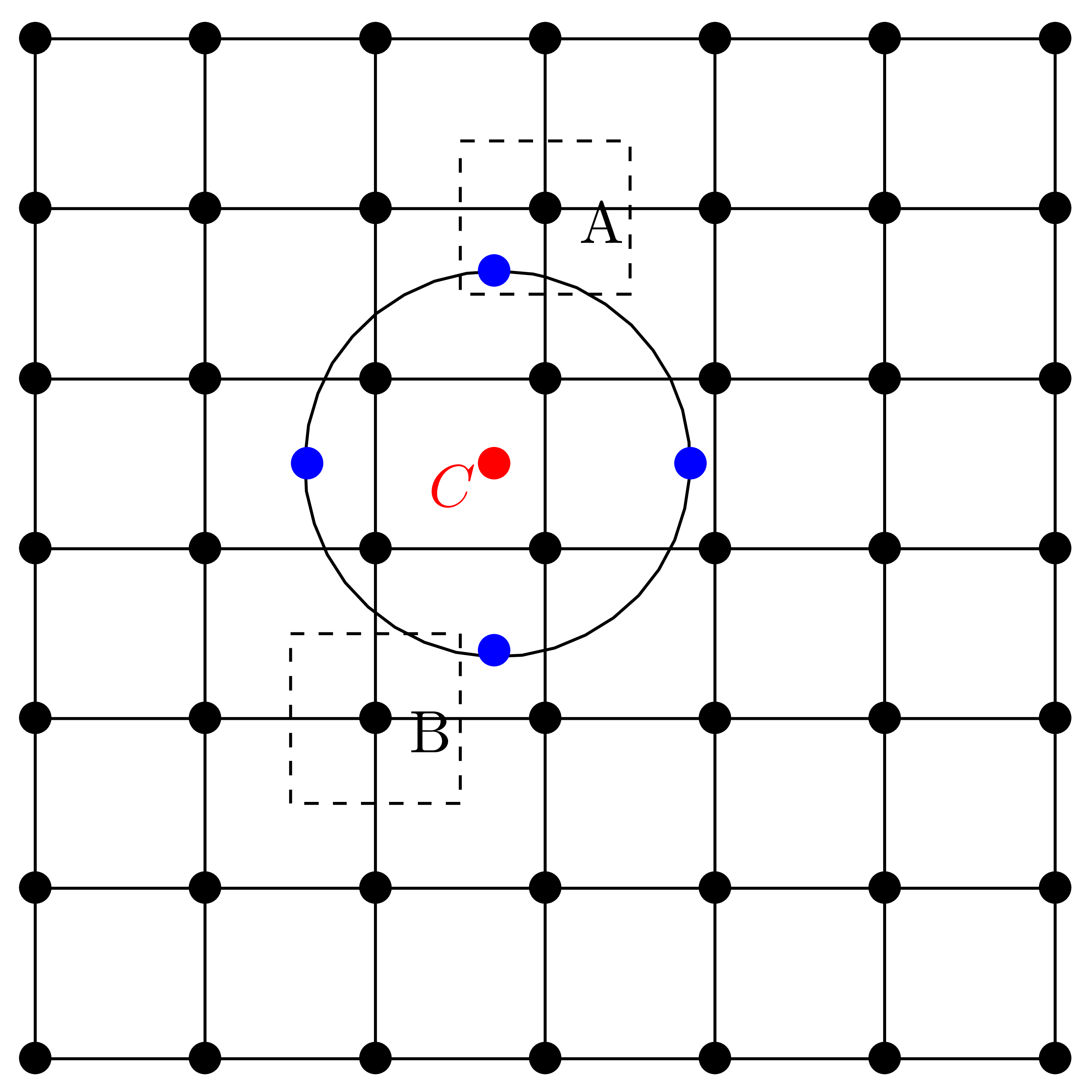 |
|
Figure 14. The spatial grid in the
plane perpendicular to the equilibrium magnetic field, a
guiding-center marker  ,
and its gyro-ring with 4 sampling points
(sub-markers) on it. The 4 sub-markers are calculated by using
the transformation (29) (inverse guiding-center
transform). Assume that Monte-Carlo weight of the guiding-center
marker is . Then The Monte-Carlo
weight of each sub-marker is ,
and its gyro-ring with 4 sampling points
(sub-markers) on it. The 4 sub-markers are calculated by using
the transformation (29) (inverse guiding-center
transform). Assume that Monte-Carlo weight of the guiding-center
marker is . Then The Monte-Carlo
weight of each sub-marker is  .
The value of integration (364) at a grid point is
approximated by .
The value of integration (364) at a grid point is
approximated by  ,
where ,
where  is the Monte-Carlo integration of
all sub-markers (associated with all guiding-center markers) in
the cell, is the Monte-Carlo integration of
all sub-markers (associated with all guiding-center markers) in
the cell,  is the cell volume. The cell
associated with a grid-point (e.g., is the cell volume. The cell
associated with a grid-point (e.g.,  ) is indicated by the dashed rectangle (this
is for the 2D projection, the cell is 3D and it is a cube). If
the Dirac delta function is used as the shape function of the
sub-markers, then calculating the contribution of a sub-marker
to a grid corresponds to the nearest-point interpolation (for
example, the 4 sub-markers will contribute nothing to grid point ) is indicated by the dashed rectangle (this
is for the 2D projection, the cell is 3D and it is a cube). If
the Dirac delta function is used as the shape function of the
sub-markers, then calculating the contribution of a sub-marker
to a grid corresponds to the nearest-point interpolation (for
example, the 4 sub-markers will contribute nothing to grid point
 since no-sub marker is located within
the cell). In practice, the flat-top shape function with its
support equal to the cell size is often used, then the
depositing corresponds to linearly interpolating the weight of
each sub-marker to the nearby grids. since no-sub marker is located within
the cell). In practice, the flat-top shape function with its
support equal to the cell size is often used, then the
depositing corresponds to linearly interpolating the weight of
each sub-marker to the nearby grids.
|
In summary, the phase-space to be sampled in gyrokinetic simulations are
still 6D rather than 5D. In this sense, the statement that gyrokinetic
simulation works in a 5D phase space is misleading. We are still working
in the 6D phase-space. The only subtle thing is that the sixth
dimension, i.e., gyro-angle, can be sampled in an easy way that is
independent of the other 5 variables.
In numerical implementation, the gyro-angle may not be explicitly used.
We just try to find 4 arbitrary points on the gyro-ring that are easy to
calculate. Some codes (e.g. ORB5) introduces a random variable to rotate
these 4 points for different markers so that the gyro-angle can be
sampled less biased.
From the view of particle simulations, the gyrokinetic model can be
considered as a noise reduction method, where the averaging over the
gyro-angle is equivalent to a time averaging over a gyro-period, which
reduces the fluctuation level (in both time and space) associated with
evaluating the Monte-Carlo phase integration. Here the averaging in
gyrokinetic particle simulation refers to taking several points on a
gyro-ring when depositing markers to spatial grids to obtain the density
and current on the grids. (Another gyro-averaging appears in evaluating
the guiding-center drift.) In gyrokinetic particle simulation, even a
step size smaller than a gyro-period is taken, the quantities used in
the model is still the ones averaged over one gyro-period. In this
sense, a gyrokinetic simulation is only meaningful when the time step
size is larger than one gyro-period. [**Some authors may disagree with
that the gyro-averaging is a time-averaging. They may consider the
gyro-averaging as the phase-space integration over the gyro-angle
coordinate. This view seems to be right in Euler simulations but seems
to be wrong in particle simulations. The reason is as follows. For each
marker, choose a random gyro-phase and then do the inverse
transformation to obtain particle position, and sum over all markers
(this corresponds to phase-space Monte-Carlo integration, which include
the gyro-angle integration, so no further gyro-angle integration is
needed); choose another random gyro-phase and repeat the above procedure
(this can be interpreted as do the phase-space Monte-Carlo integration
at another time), choose further random gyro-phase for each marker and
repeat. Finally averaging all the above values to obtain the final
estimation of the phase-space integration. This amounts to a
time-averaging over a gyro-motion. In summary, sampling several times
with different gyro-phases for each marker and taking the average
amounts to the time averaging over gyro-motion**]
When doing the time-average over the ion cyclotron motion, the time
variation of the low-frequency mode is negligible and only the spatial
variation of the modes is important. For the gyro-motion, only the
gyro-angle is changing and all the other variables, , are approximately constant. As a result,
this time averaging finally reduces to a gyro-averaging.
I prefer to reason in terms of particle position and velocity, and
consider the guiding-center location as an image of the particle
position. When working in the guiding-center coordinates, I prefer to
reason by transforming back to the particle position. This reasoning is
clear and help me avoid some confusions I used to have.
In coding, the initial sampling of the phase space is performed for
particles ( of particles) and then is transformed
to guiding-center coordinates.
of particles) and then is transformed
to guiding-center coordinates.
E.4Distribution function transform**check
In the above, we assume that and are related to each other by the guiding-center
transformation (27) or (29) , i.e., and are not independent. For some
cases, it may be convenient to treat and as independent variables and express the
guiding-center transformation via an integral of the Dirac delta
function. For example,
 |
(359) |
where and are considered
as independent variables, is the gyroradius
evaluated at ,  is the three-dimensional Dirac delta function. [In terms
of general coordinates
is the three-dimensional Dirac delta function. [In terms
of general coordinates  , the
three-dimensional Dirac delta function is defined via the 1D Dirac delta
function as follows:
, the
three-dimensional Dirac delta function is defined via the 1D Dirac delta
function as follows:
 |
(360) |
where  is the the Jacobian of the general
coordinate system. The Jacobian is included in order to make
is the the Jacobian of the general
coordinate system. The Jacobian is included in order to make  satisfy the normalization condition
  .]
.]
Expression (359) can be considered as a transformation that
transforms an arbitrary function from the guiding-center coordinates to
the particle coordinates. Similarly,
 |
(361) |
is a transformation that transforms an arbitrary function from the the
particle coordinates to the guiding-center coordinates.
E.5Moments of distribution function expressed
as integration over guiding-center variables
In terms of particle variables ,
it is straightforward to calculate the moment of the distribution
function. For example, the number density  is
given by
is
given by
 |
(362) |
However, it is a little difficult to calculate
at real space location by using the
guiding-center variables .
This is because holding constant and changing
, which is required by the
integration in Eq. (362), means the guiding-center variable
is changing according to Eq. (27).
Using Eq. (34), expression (362) is written as
 |
(363) |
As is mentioned above, the  integration in Eq.
(363) should be performed by holding
constant and changing , which
means the guiding-center variable
integration in Eq.
(363) should be performed by holding
constant and changing , which
means the guiding-center variable  is changing.
This means that, in space, the above integration
is a (generalized) curve integral along the the curve
is changing.
This means that, in space, the above integration
is a (generalized) curve integral along the the curve  with being constant. Treating
and as independent variables and using the Dirac
delta function
with being constant. Treating
and as independent variables and using the Dirac
delta function  , this curve
integral can be written as the following double integration over the
independent variables and :
, this curve
integral can be written as the following double integration over the
independent variables and :
 |
(364) |
Another perspective of interpreting Eq. (364) is that we
are first using the transformation (359) to transform to and then integrating in the velocity space.
FDiamagnetic flow
**check**
The perturbed distribution function given in Eq.
() contains two terms. The first term is gyro-phase dependent while the
second term is gyro-phase independent. The perpendicular velocity moment
of the second term will give rise to the so-called diamagnetic flow. For
this case, it is crucial to distinguish between the distribution
function in terms of the guiding-center variables,  , and that in terms of the particle variables,
 . In terms of these
denotations, equation () is written as
. In terms of these
denotations, equation () is written as
 |
(365) |
Next, consider the perpendicular flow  carried by
. This flow is defined by the
corresponding distribution function in terms of the particle variables,
carried by
. This flow is defined by the
corresponding distribution function in terms of the particle variables,
 , via,
 |
(366) |
where is the number density defined by  . Using the relation between the
particle distribution function and guiding-center distribution function,
equation (366) is written as
. Using the relation between the
particle distribution function and guiding-center distribution function,
equation (366) is written as
 |
(367) |
Using the Taylor expansion near ,
 can be approximated as
 |
(368) |
Plugging this expression into Eq. (367), we obtain
 |
(369) |
As mentioned above,  is independent of the
gyro-angle . It is obvious
that the first integration is zero and thus Eq. (369) is
reduced to
is independent of the
gyro-angle . It is obvious
that the first integration is zero and thus Eq. (369) is
reduced to
 |
(370) |
Using the definition  , the
above equation is written
, the
above equation is written
where  , which is independent
of the gyro-angle because both
and are independent of . Next, we try to perform the integration over in Eq. (371). In terms of velocity space
cylindrical coordinates
, which is independent
of the gyro-angle because both
and are independent of . Next, we try to perform the integration over in Eq. (371). In terms of velocity space
cylindrical coordinates  ,
is written as
,
is written as
 |
(372) |
where  and
and  are two
arbitrary unit vectors perpendicular each other and both perpendicular
to
are two
arbitrary unit vectors perpendicular each other and both perpendicular
to  .
.  can be written as
 |
(373) |
where  and
and  are
independent of . Using these
in Eq. (371), we obtain
are
independent of . Using these
in Eq. (371), we obtain
Using  , the above equation is
written as
, the above equation is
written as
where
is the perpendicular pressure carried by .
The flow given by Eq. (375) is called the diamagnetic flow.
GTransform gyrokinetic equation from to  coordinates
The gyrokinetic equation given above is written in terms of variables
. Next, we transform it into
coordinates  which are defined by
 |
(377) |
Use this definition and the chain rule, we obtain
and
Then, in terms of , equation
(135) is written
|
|
 |
|
|
|
 |
(380) |
Dropping terms of order higher than ,
equation (380) is written as
|
|
 |
|
|
|
 |
(381) |
The above equation drops all terms higher than
and as a result the coefficient before  contains
only the mirror force, i.e.,
contains
only the mirror force, i.e.,  ,
which is independent of any perturbations.
,
which is independent of any perturbations.
Note that the gyro-averaging operator in
coordinates is identical to that in the old coordinates since the
perpendicular velocity variable is identical
between the two coordinate systems. Also note that the perturbed
guiding-center velocity is given by
 |
(382) |
where (rather than  )
is used. Since
)
is used. Since  , which is
independent of , then Eq. (378) indicates that
, which is
independent of , then Eq. (378) indicates that  .
.
Following the same procedures, equation (143) in terms of
is written as
next, try to recover the equation in Mishchenk's paper:

,
 |
(384) |


G.1Recover equation in W. Deng's 2011 NF
paper
The guiding-center velocity in the equilibrium field is given by
 |
(385) |
where
 |
(386) |
 |
(387) |
Using  , then expression (385) is written as
 |
(388) |
where the curvature drift,  drift, and drift can be identified. Note that the perturbed
guiding-center velocity is given by (refer to
Sec. C.3)
drift, and drift can be identified. Note that the perturbed
guiding-center velocity is given by (refer to
Sec. C.3)
 |
(389) |
Using the above results, equation (383) is written as
Collecting coefficients before  ,
we find that the two terms involving
,
we find that the two terms involving  (terms in
blue and red) cancel each other, yielding
(terms in
blue and red) cancel each other, yielding
This equation agrees with Eq. (8) in I. Holod's 2009 pop paper
(gyro-averaging is wrongly omitted in that paper) and W. Deng's 2011 NF
paper.
HDrift-kinetic limit
In the drift-kinetic limit,  ,
,
 , and
, and  , where is an arbitrary
field quantity. Using these, gyrokinetic equation (347) is
written as
, where is an arbitrary
field quantity. Using these, gyrokinetic equation (347) is
written as
|
|
 |
|
|
|
 |
(392) |
H.1Linear case
Neglecting the nonlinear terms, drift-kinetic equation (392)
is written
|
|
 |
|
|
|
 |
(393) |
Next let us derive the parallel momentum equation from the linear drift
kinetic equation (this is needed in my simulation). Multiplying the
linear drift kinetic equation (393) by  and then integrating over velocity space, we obtain
Equation (394) involve  and this
should be avoided in particle methods whose goal is to avoid directly
evaluating the derivatives of over phase-space
coordinates. On the other hand, the partial derivatives of velocity
moment of are allowed. Therefore, we would like
to make the velocity integration of appear. Note
that here is taken by holding
constant and thus is not a constant and thus can
not be moved inside . Next,
to facilitate performing the integration over , we transform the linear drift kinetic equation (393) into variable
and this
should be avoided in particle methods whose goal is to avoid directly
evaluating the derivatives of over phase-space
coordinates. On the other hand, the partial derivatives of velocity
moment of are allowed. Therefore, we would like
to make the velocity integration of appear. Note
that here is taken by holding
constant and thus is not a constant and thus can
not be moved inside . Next,
to facilitate performing the integration over , we transform the linear drift kinetic equation (393) into variable  .
.
H.2Transform from  to coordinates
The kinetic equation given above is written in terms of variable . Next, we transform it into
coordinates  which is defined by
 |
(395) |
 |
(396) |
and
 |
(397) |
Use this, we have
and
Then, in terms of variable  ,
equation (393) is written
,
equation (393) is written
|
|
 |
|
|
|
 |
(400) |
where  .
.
H.3Parallel momentum equation
Multiplying the linear drift kinetic equation (400) by and then integrating over velocity space, we obtain
Consider the simple case that does not carry
current, i.e.,  is an even function about . Then it is obvious that the
integration of the terms in red in Eq. (401)
are all zero. Among the rest terms, only the following term
is an even function about . Then it is obvious that the
integration of the terms in red in Eq. (401)
are all zero. Among the rest terms, only the following term
 |
(402) |
explicitly depends on . Using
 , the integration in the
above expression can be analytically performed, giving
, the integration in the
above expression can be analytically performed, giving
Using these results, the parallel momentum equation (401)
is written
where the explicit dependence on is via the
first term  , with all the the
other terms being explicitly independent of
( and
, with all the the
other terms being explicitly independent of
( and  implicitly depend
on ).
implicitly depend
on ).
Equation (404) involve derivatives of
with respect to space and and these should be
avoided in the particle method whose goal is to avoid directly
evaluating these derivatives. Using integration by parts, the terms
involving  can be simplified, yielding
Define  and
and  ,
then the above equation is written
,
then the above equation is written
Next, we try to eliminate the spatial gradient of
by changing the order of integration. The second term on the right-hand
side of Eq. (406) is written
where  . Similarly, the term
 is written as
where  . Similarly, the term
 can be written as the gradient of moments of
. Let us work on this. The
drift
can be written as the gradient of moments of
. Let us work on this. The
drift  is given by
 |
(409) |
where  (refer to my another notes). Using
  , we obtain
  . Then is written

Using this and  , the term
is written as
, the term
is written as
which are the third order moments of and may be
neglect-able (a guess, not verified). Using the above results, the
linear parallel momentum equation is finally written
Define
 |
(412) |
which, for the isotropic case ( ),
is simplified to
),
is simplified to
 |
(413) |
then Eq. (411) is written as
H.4Special case in uniform magnetic field
In the case of uniform magnetic field, the parallel momentum equation
(411) is written as
 |
(415) |
H.5Electron perpendicular flow
Using the gyrokinetic theory and taking the drift-kinetic limit, the
perturbed perpendicular electron flow,  ,
is written (see Sec. F or Appendix in Yang Chen's paper[1])
,
is written (see Sec. F or Appendix in Yang Chen's paper[1])
 |
(416) |
where is the equilibrium electron number
density,  is the perturbed perpendicular pressure
of electrons.
is the perturbed perpendicular pressure
of electrons.
H.5.1Drift kinetic equation
Drift kinetic equation is written
 |
(417) |
where  ,
,  is the magnetic moment,
  ,
,
 is the unit vector along the equilibrium
magnetic field,
is the unit vector along the equilibrium
magnetic field,  is the guiding-center drift in
the equilibrium magnetic field. and are the perturbed electric field and magnetic field,
respectively.
is the guiding-center drift in
the equilibrium magnetic field. and are the perturbed electric field and magnetic field,
respectively.
H.5.2Parallel momentum equation
Multiplying the drift kinetic equation () by and
then integrating over velocity space, we obtain
 |
(418) |
which can be written as
 |
(419) |
Using  , the last term on the
RHS of the above equation is written
, the last term on the
RHS of the above equation is written
where use has been made of  .
.
 |
(422) |
Using Eq. () in Eq. (), we obtain
 |
(423) |
————–
 |
(424) |
ddddd

IDerivation of Eq. (122),
not finished
From the definition of , we
obtain
 |
(425) |
Using
 |
(426) |
expression (425) is written as
 |
(427) |
which agrees with Eq. (10) in Frieman-Chen's paper[3].


Using the fact that is independent of , the left-hand side of Eq. (122) is written as

JModern gyrokinetic formulation
Frimain-Chen equation was obtained by first transforming to the
guiding-center coordinates and then using the classical perturbation
expansion for the distribution function (to separate gyro-phase
independent part form the gyro-phase dependent one). Note that the
guiding-center transform does not involve the perturbed field.
The modern form of the nonlinear gyrokinetic equation is in the total-f
form. This way of deriving the gyrokinetic equation is to use coordinate
transforms to eliminate gyro-phase dependence of the total distribution
function (rather than splitting the distribution function itself) and
thus obtain an equation for the resulting gyro-phase independent
distribution function (called gyro-center distribution function). The
coordinate transform involves the perturbed fields besides the
equilibrium field.
The resulting equation for the gyro-center distribution function is
given by (see Baojian's paper)
 |
(428) |
where
 |
(429) |
 |
(430) |
Here the independent variables are gyro-center position , magnetic moment and
parallel velocity .
The gyro-phase dependence of the particle distribution can be recovered
by the inverse transformation of the transformation used before. The
pull-back transformation (inverse gyro-center transform) gives rise to
the polarization density term. (phase-space-Lagrangian Lie perturbation
method (Littlejohn, 1982a, 1983), I need to read these two papers.).
The learning curve of Lie tansform gyrokinetic theory seems steep. I
tried to learn it but failed. To derive the Frieman-Chen equation, you
just need some patience. Meanwhile, patience is all that you need to
learn any mathematic stuff, but some requires more patience than others,
and Lie transform gyrokinetic is one that requires more for me.
9About this document
These notes were initially written when I visited University of Colorado
at Boulder (Sept.-Nov. 2016), where I worked with Yang Chen, who said
that most gyrokinetic simulations essentially employ Frieman-Chen's
equation. So a careful re-derivation of the equation is highly helpful
for one who is interested in implementing gyrokinetic models in codes,
which motivated me to write this document.
After the visit, I went to CUB again, working with Yang Chen and Scott
Parker as a postdoc researcher for two years, during which I tried to
develop a fully kinetic code (including gyromotion of ions and
drift-kinetic electrons) for electromagnetic turbulence simulation. I
got an electrostatic version (fully kinetic ions with adiabatic
electrons) work[5], but failed to deliver a working
electromagnetic version. After coming back to ASIPP, I transformed that
code to a gyrokinetic code (gyrokinetic ions with drift-kinetic
electrosn), which can handle electromagnetic perturbations (using the
mixed-variable pull-back method). That is the TEK code
discussed in the main text.
This document was written by using TeXmacs[9], a structured
wysiwyw (what you see is what you want) editor for scientists. The HTML
version of this document is generated by using TeXmacs' HTML converter.
Bibliography
-
[1]
-
Yang Chen and Scott E. Parker. Particle-in-cell
simulation with vlasov ions and drift kinetic electrons.
Phys. Plasmas, 16:52305, 2009.
-
[2]
-
A. M. Dimits, G. Bateman, M. A. Beer, B. I. Cohen, W.
Dorland, G. W. Hammett, C. Kim, J. E. Kinsey, M.
Kotschenreuther, A. H. Kritz, L. L. Lao, J. Mandrekas, W. M.
Nevins, S. E. Parker, A. J. Redd, D. E. Shumaker, R. Sydora, and
J. Weiland. Comparisons and physics basis of tokamak transport
models and turbulence simulations. Physics of Plasmas,
7(3):969–983, 2000.
-
[3]
-
E. A. Frieman and Liu Chen. Nonlinear gyrokinetic
equations for low-frequency electromagnetic waves in general
plasma equilibria. Physics of Fluids,
25(3):502–508, 1982.
-
[4]
-
T. Görler, N. Tronko, W. A. Hornsby, A. Bottino,
R. Kleiber, C. Norscini, V. Grandgirard, F. Jenko, and E.
Sonnendrücker. Intercode comparison of gyrokinetic global
electromagnetic modes. Physics of Plasmas, 23(7):72503,
2016.
-
[5]
-
Youjun Hu, Matthew T. Miecnikowski, Yang Chen, and
Scott E. Parker. Fully kinetic simulation of
ion-temperature-gradient instabilities in tokamaks.
Plasma, 1(1):105–118, 2018.
-
[6]
-
X. Lapillonne, B. F. McMillan, T. Görler, S.
Brunner, T. Dannert, F. Jenko, F. Merz, and L. Villard.
Nonlinear quasisteady state benchmark of global gyrokinetic
codes. Physics of Plasmas, 17(11):112321, 2010.
-
[7]
-
A. Mishchenko, A. Bottino, A. Biancalani, R. Hatzky,
T. Hayward-Schneider, N. Ohana, E. Lanti, S. Brunner, L.
Villard, M. Borchardt, R. Kleiber, and A. Könies. Pullback
scheme implementation in orb5. Computer Physics
Communications, 238:194–202, 2019.
-
[8]
-
Benjamin J. Sturdevant, S. Ku, L. Chacón, Y.
Chen, D. Hatch, M. D. J. Cole, A. Y. Sharma, M. F. Adams, C. S.
Chang, S. E. Parker, and R. Hager. Verification of a fully
implicit particle-in-cell method for the v ∥-formalism of
electromagnetic gyrokinetics in the xgc code. Physics of
Plasmas, 28(7):72505, jul 2021.
-
[9]
-
Joris van der Hoeven. Gnu texmacs, a structured
wysiwyw (what you see is what you want) editor for scientists.
http://www.texmacs.org/, 2007. [Online].


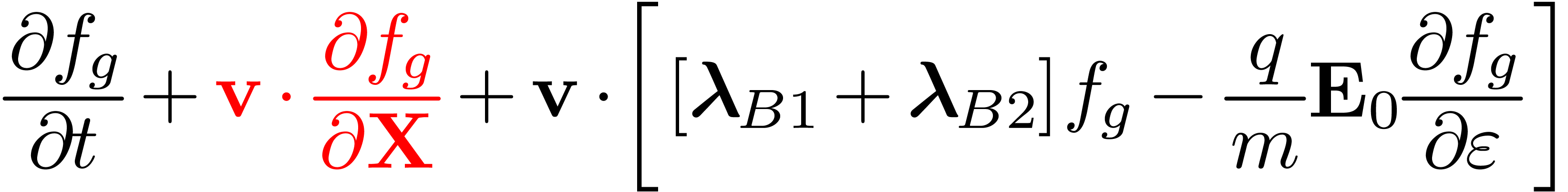
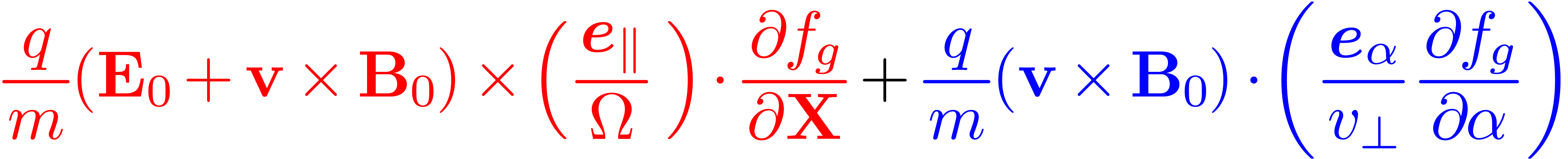


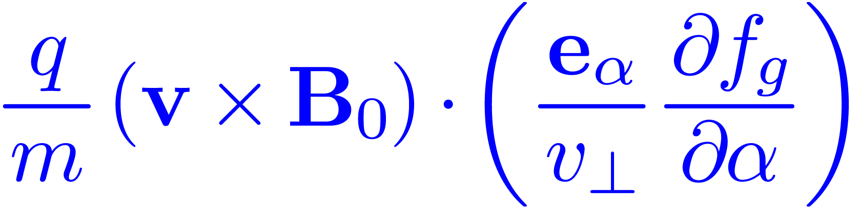


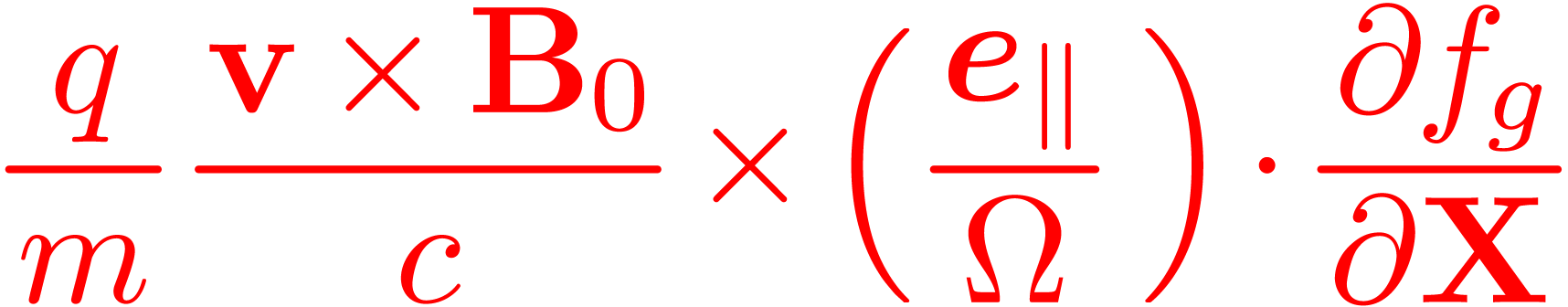


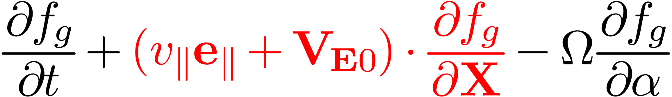


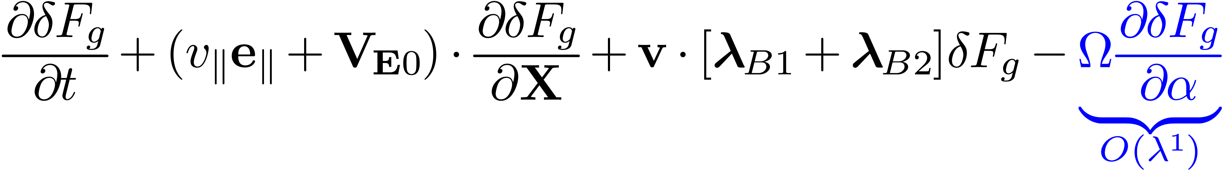


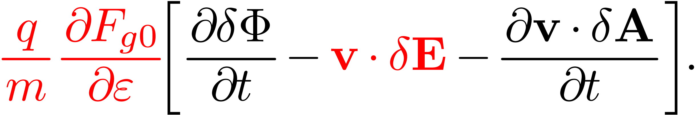

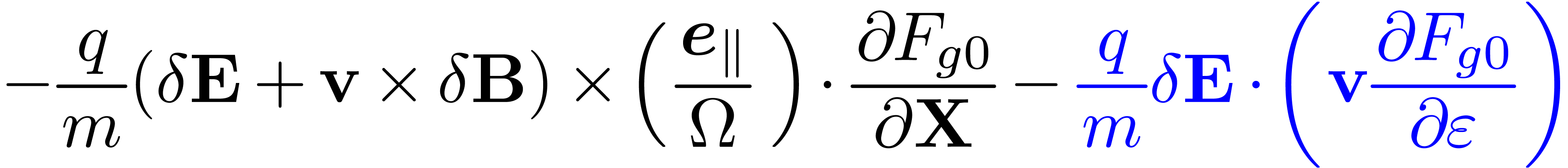

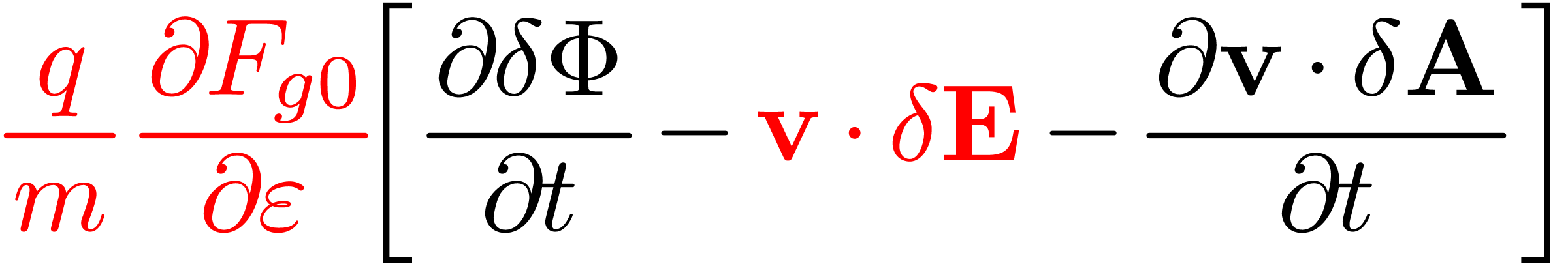


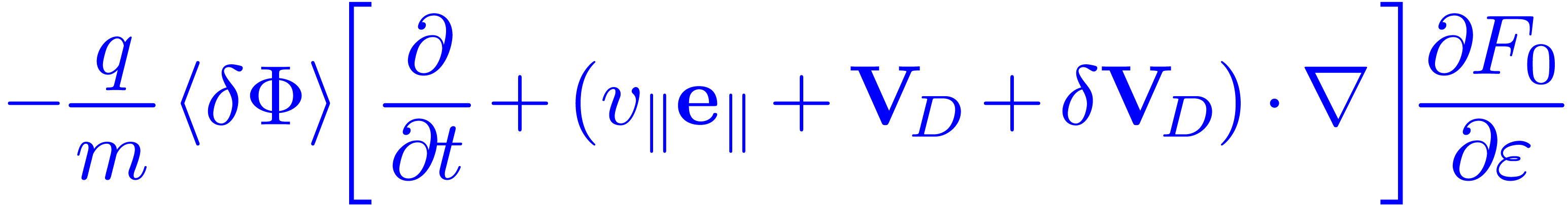


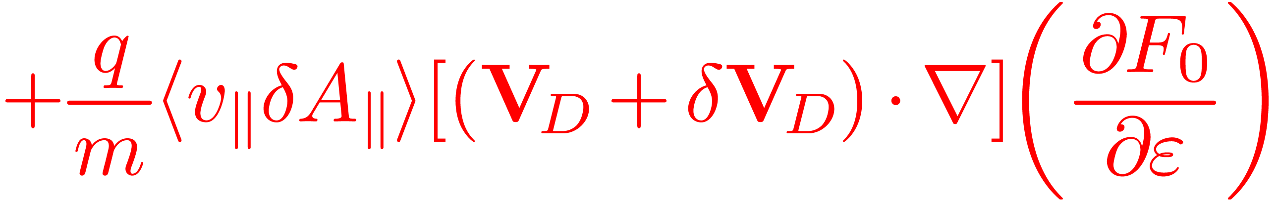


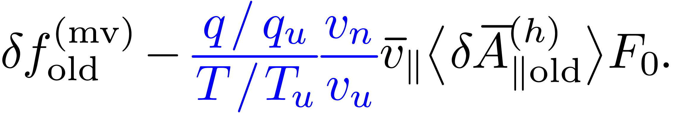


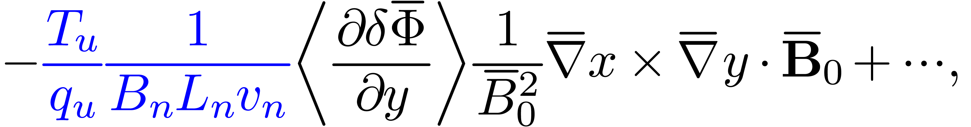


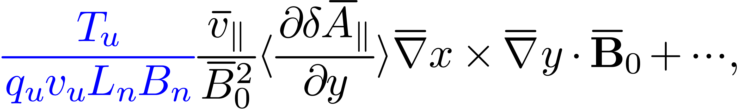

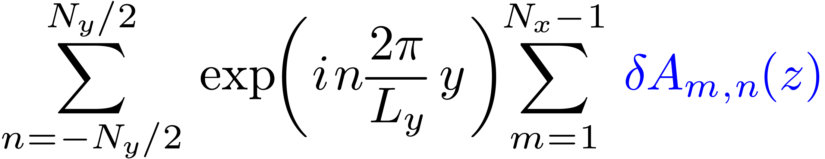


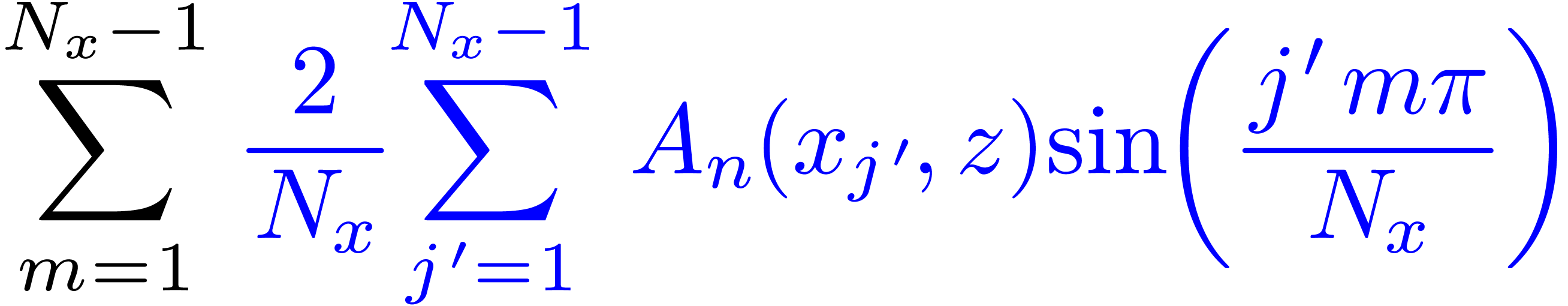

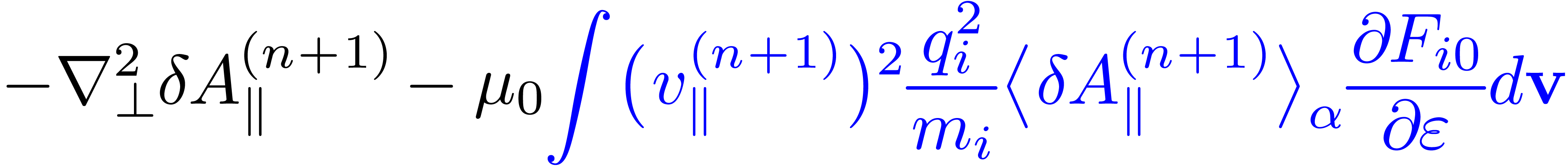
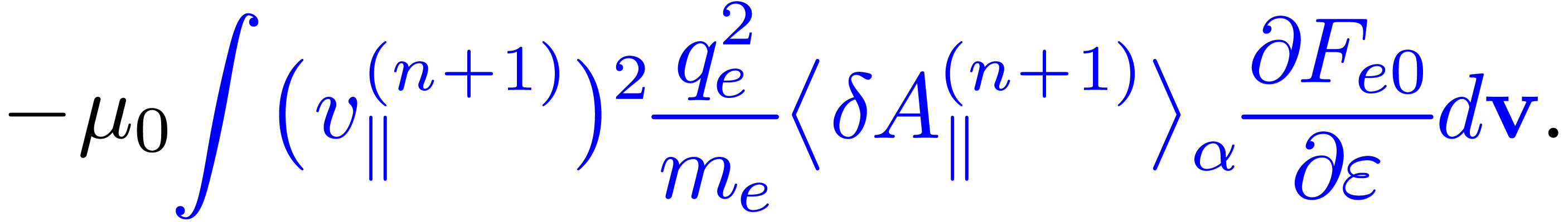

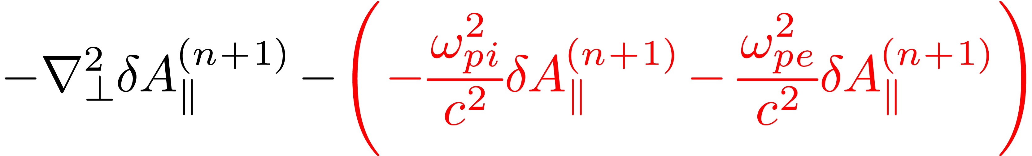


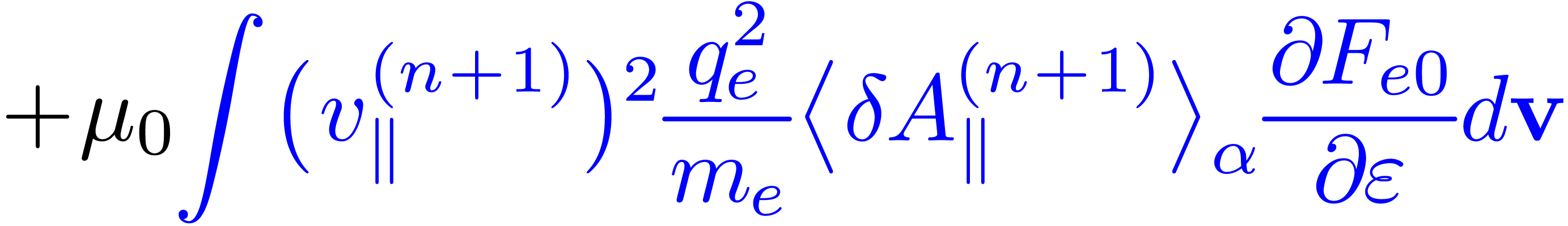
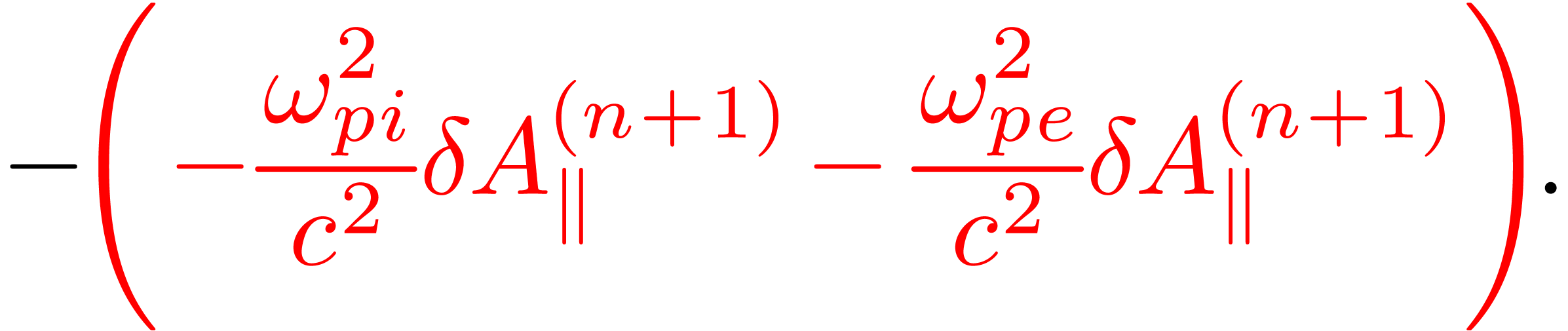


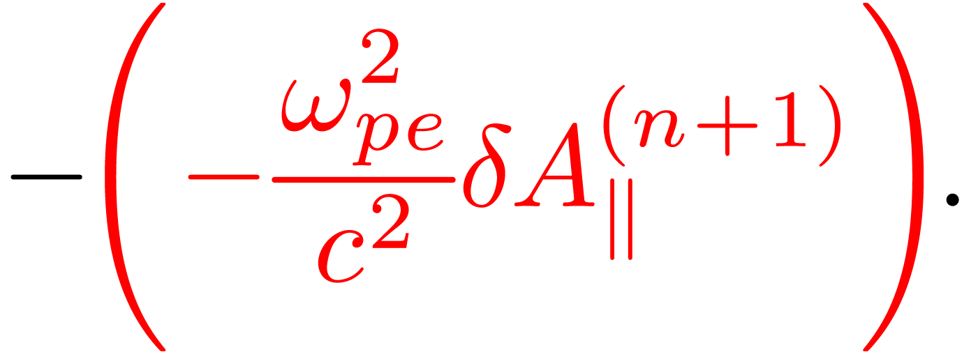

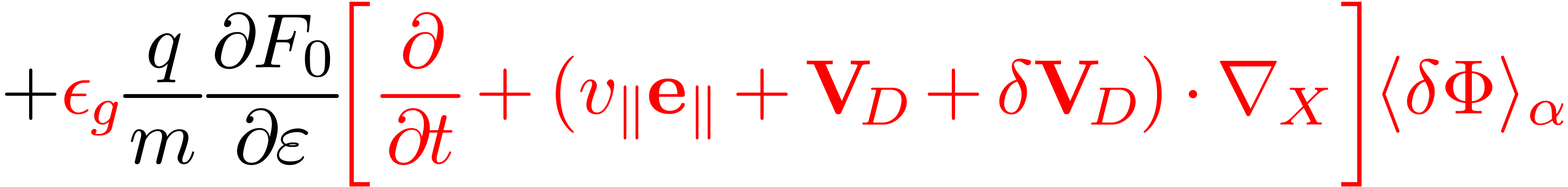
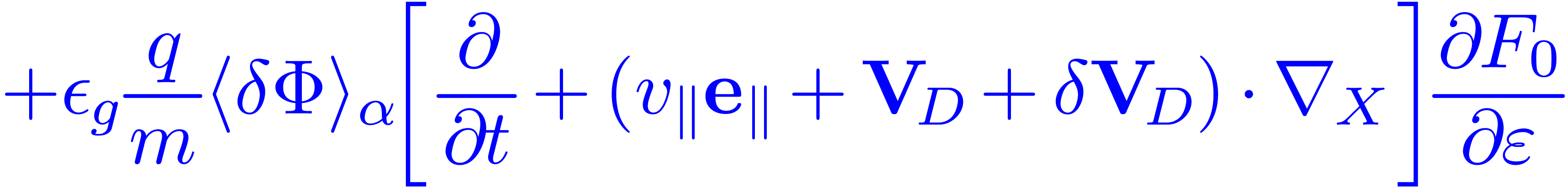


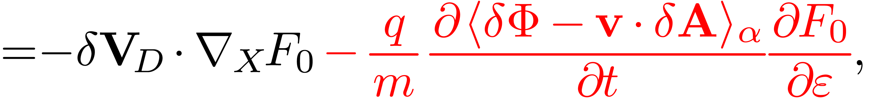
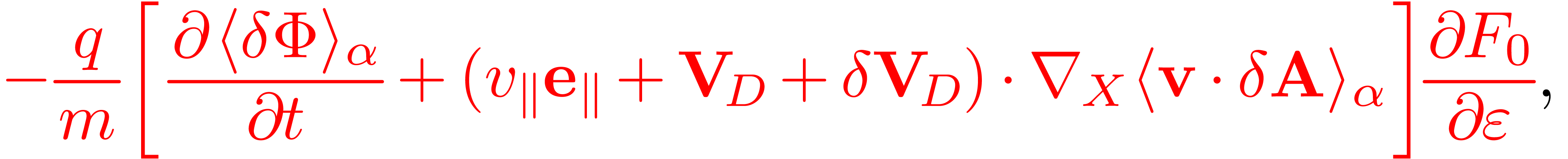


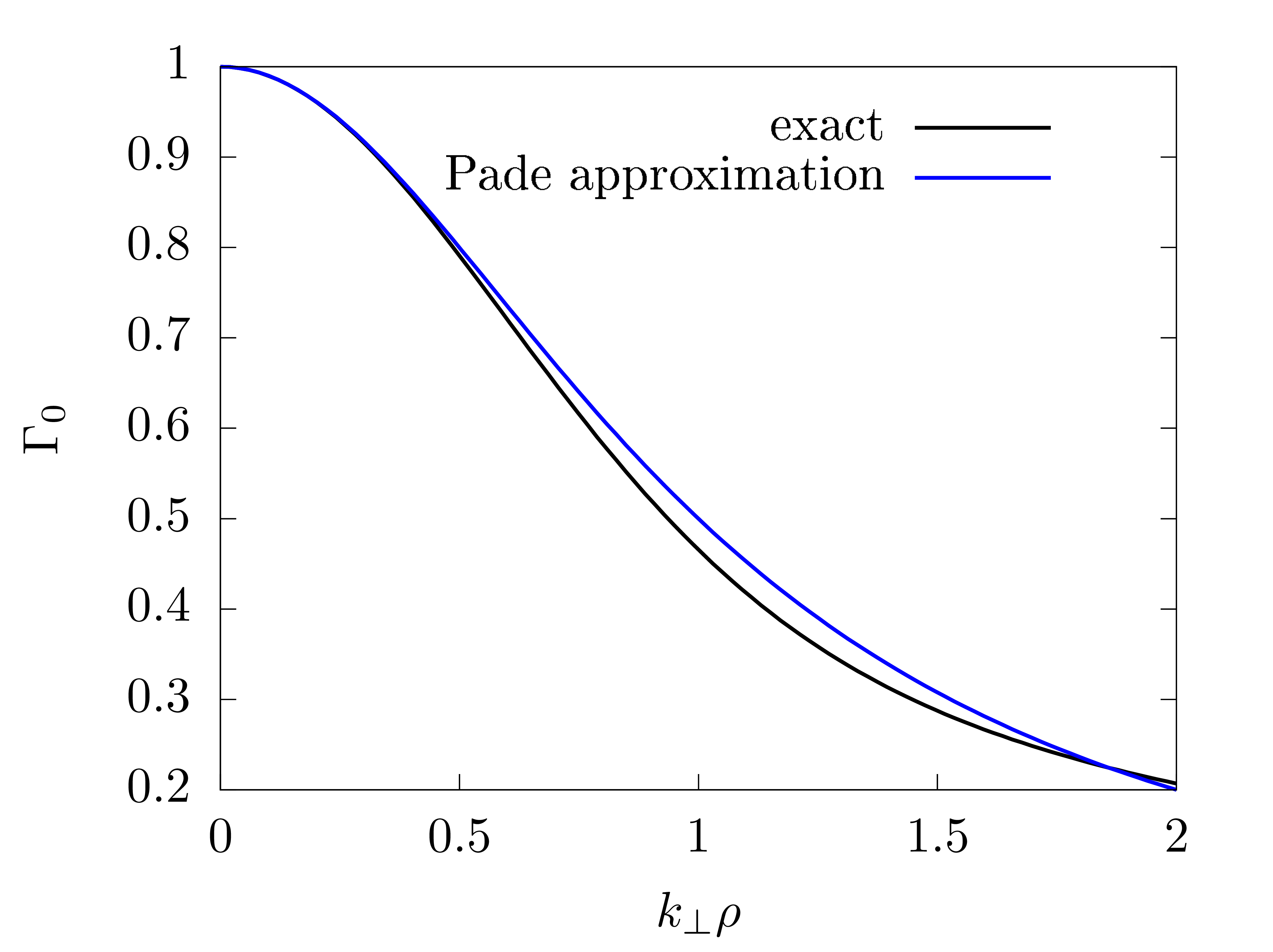
 and the corresponding
Pade approximation
and the corresponding
Pade approximation  .
.


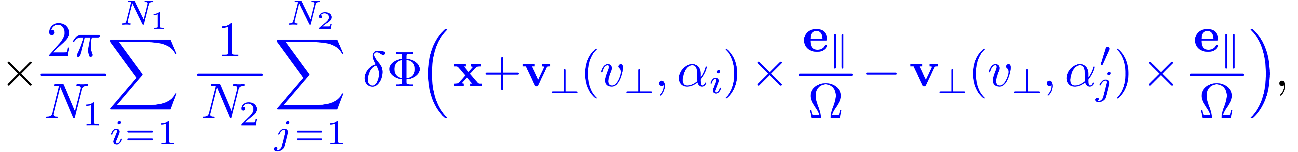
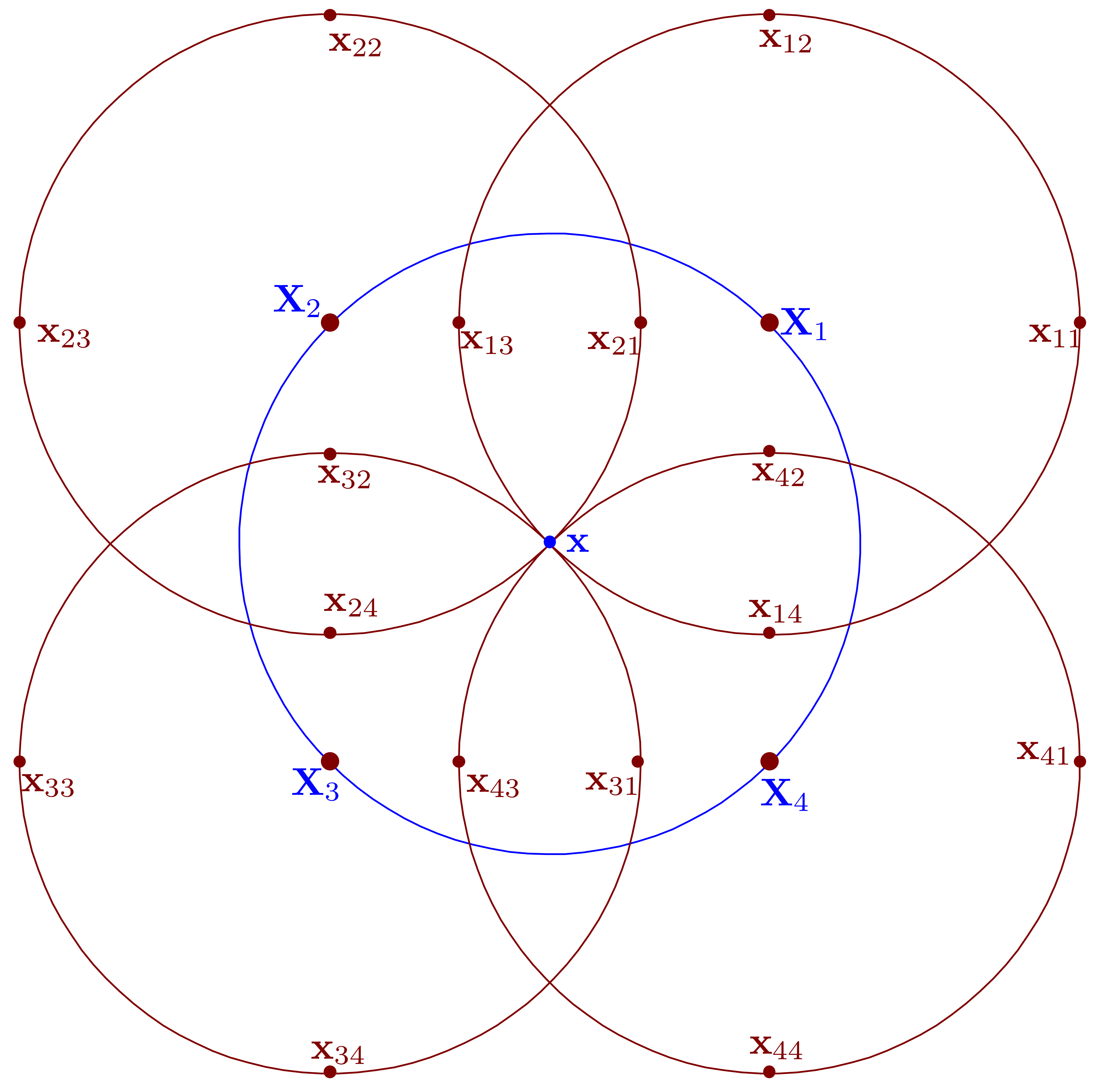
 and
and  with
with  ,
, with
with  with
with  ,
,
 for the case shown in Fig.

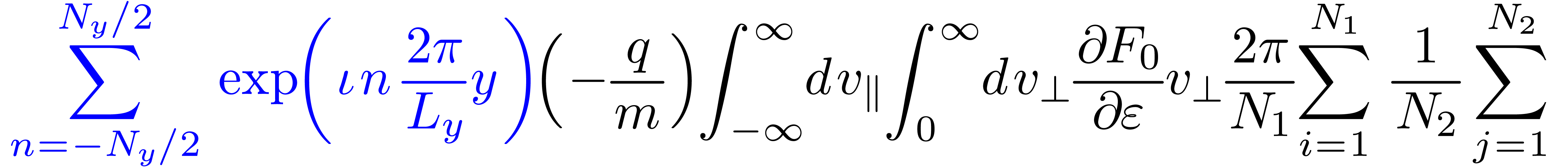


 is the minor radius of the
last-closed-flux-surface,
is the minor radius of the
last-closed-flux-surface,  ,
, at
at  is assumed to be a constant independent of
  ,
, .
. and
and  .
. is the thermal ion gyro-radius,
 is the ion cyclotron angular frequency
at the magnetic axis.
is the ion cyclotron angular frequency
at the magnetic axis.
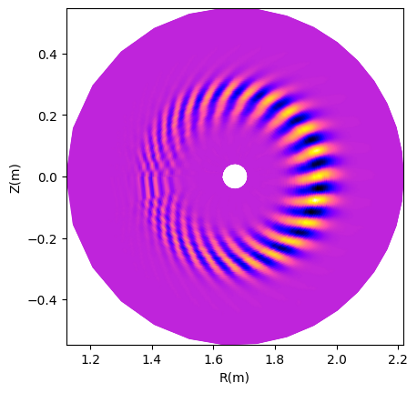
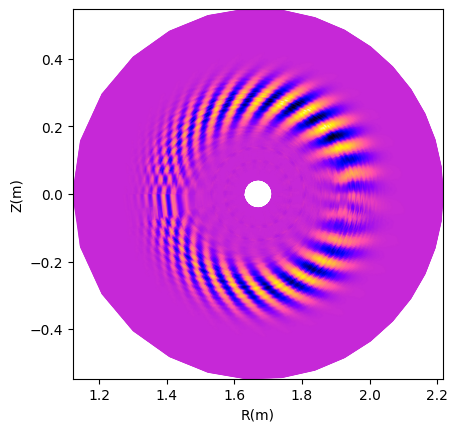
 ,
, ,
,
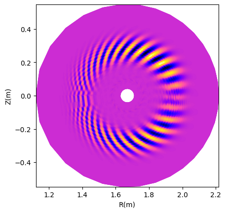
 for
for 
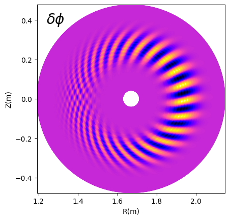
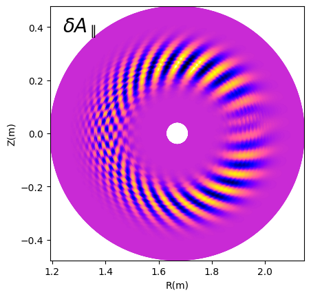
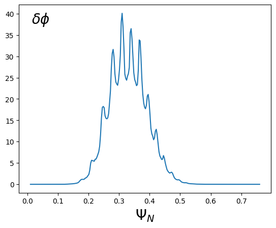
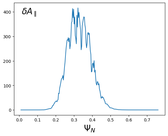
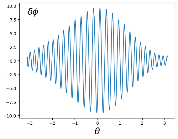
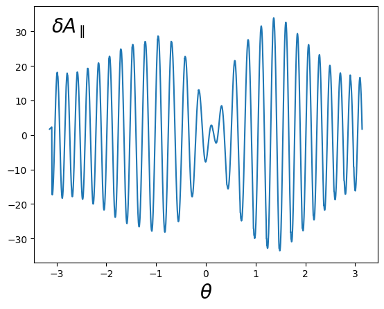
 .
.


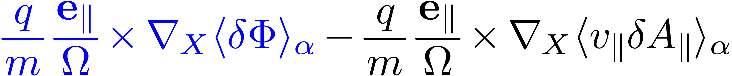

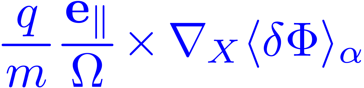


 .
. is increasing along the anti-clockwise
direction when viewed along
is increasing along the anti-clockwise
direction when viewed along  direction with
 is the toroidal angle of the right-handed
cylindrical coordinates
is the toroidal angle of the right-handed
cylindrical coordinates  .
.
 and ends at
  (
( is chosen to be at the high-field side
midplane in both the codes). TEK array index starts
from 1 whereas GEM array index starts from
is chosen to be at the high-field side
midplane in both the codes). TEK array index starts
from 1 whereas GEM array index starts from  .
. .
.
 and
and 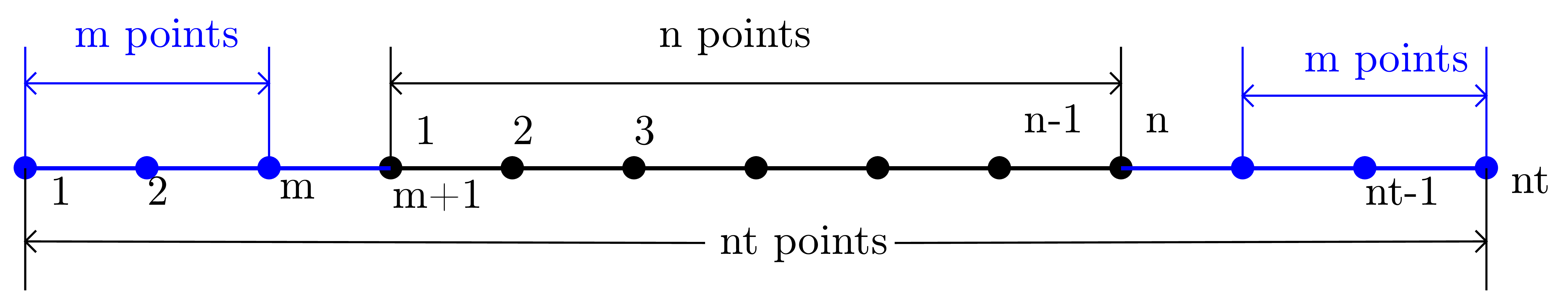
 ,
, is the number of grid points in one of the two
buffer regions (regions in blue color). In the code
is the number of grid points in one of the two
buffer regions (regions in blue color). In the code  is denoted by nflux2 and
  is denoted by nflux,