1 Equations of guiding-center motion

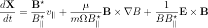
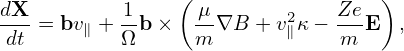
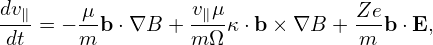
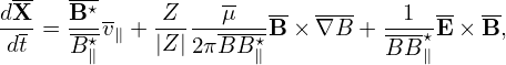
The equations of guiding center motion are given by[1]

(1)

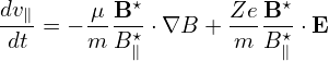(2)

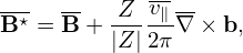
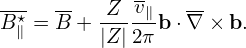
where X is the guiding-center position, v_∥ is the parallel (to the magnetic field) velocity defined by v_∥ = B⋅v∕B; Here m, Ze, and v are the mass, charge and velocity of the particle, respectively, μ is the magnetic moment defined by μ = mv_⊥²∕(2B) with v_⊥ being the perpendicular speed; Ω = BZe∕m is the cyclotron angular frequency,  B^⋆ and B_∥^⋆ are defined by

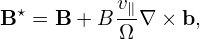(3)

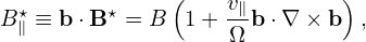(4)

respectively, where b = B∕B. If we use the approximation B_∥^⋆ ≈ B, then the drift velocity in Eq. (1) can be written as

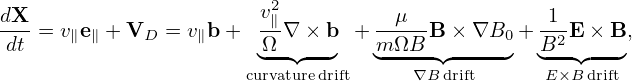(5)

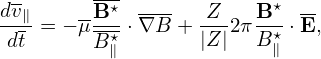
where the usual drifts can be recognized. Before getting to know the above form of the equations of the guiding-center motion, I used the following form of the equations (refer to my notes “collisionless_drift_kinetic_equation.tm”):

(6)

(7)

which does not conserve the toroidal angular momentum P_ϕ exactly in an axisymmetrical equilibrium magnetic field (this has been tested numerically) while the new form given in Eqs. (1)-(4) can conserve P_ϕ exactly. My latest numerical code uses Eqs. (1)-(4) as the the equations of guiding center motion. The toroidal angular momentum P_ϕ is defined by

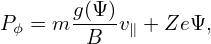(8)

where Ψ = A_ϕR with A_ϕ being the toroidal component of the magnetic vector potential.

1.1 Define new units

The above formulas are in SI units, which are good since SI units are widely used and thus these formulas are accessible to most people, making communications easier. However, many physicists prefer to define new units for a specific problem and write the equations in terms of these new units. This process is often called normalization. This has the advantage of possibly reducing the number of free parameters in a problem. Another advantage is that, by chosen proper characteristic quantities as units, the magnitude of quantities in terms of the new units are easier to be appreciated. A third advantage is that the magnitude of normalized quantities may be in the vicinity of 1 (if suitable units are chosen), and thus numerical overflow in a numerical computation may be avoided, making the computation more accurate. The disadvantages of the normalization are (1) the additional work associated with performing the transformation between two units systems, (2) possible confusions about which units are used in a numerical code and the potential of introducing bugs due to this confusion when writing or revising numerical codes.

The units I adopted are as follows. Choose a characteristic magnetic field strength B_n and a characteristic length L_n. Using B_n and L_n, we define a characteristic time t_n ≡ 2π∕Ω_n, where Ω_n = B_n|Ze|∕m, a characteristic velocity v_n = L_n∕t_n,  and a characteristic magnetic moment μ_n = mv_n²∕B_n. Using these characteristic quantities as units, I define the following normalized quantities:

(9)

In terms of the above normalized quantities, Eqs. (1)-(4) are written, respectively, as

(10)

(11)

(12)

and

(13)

In the normalized form, there is only one parameter for distinguishing particle species, namely the sign of particle’s charge Z∕|Z|. The other parameters for particle species enters via the normalization factor Ω_n = B_n|Ze|∕m.

The toroidal angular momentum P_ϕ is normalized by ZeB_nL_n².

In TEK code, I choose B_n = 1T and L_n = 1m, i.e., they are identical to the corresponding SI units. This choice makes my unit system become bad because it is hard to relate v_n defined above to any typical velocity in a tokamak plasma. A better choice would be choose B_n to the magnetic field magnitude at the magnetic axis and choose L_n to be v_t∕Ω_n, i.e., the Larmor radius of a typical particles, where v_t is the thermal velocity of a species. Then define t_n = 1∕Ω_n and define v_n by v_n = L_n∕t_n = v_t, which is a typical particle velocity. In future, I may change TEK code to using this unit system, but presently I stick to using the above unit system.