Use constants of motion to determine orbit loss

7 Use constants of motion to determine orbit loss

This section discusses determining the prompt loss of ions by using the constants of motion. This work was motivated by Dr. Chengkang Pan, who shares an oﬃce with me and recently (2014) published a NF paper discussing this topic.

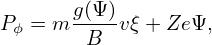
7.1 Critical velocity for ions to touch a boundary

There are three constants of motion for a guiding center drift, namely, the canonical toroidal angular momentum P_ϕ, the magnetic moment μ, and the total kinetic energy 𝜀, which are given, respectively, by

g(Ψ-) Pϕ = m B vξ + ZeΨ,

(116)

μ = m-v2(1− ξ2), B

(117)

𝜀 = 1mv2, 2

(118)

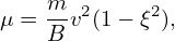
where g(Ψ) = RB_ϕ, ξ is the cosine of the pitch angle of guiding center velocity (with respect to the local magnetic ﬁeld), Ψ = RA_ϕ with A_ϕ being the toroidal component of the magnetic vector potential, Ze and m are the charge and mass of the ion, respectively.

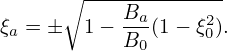
Next, we use the constraint of the three constants of motion to determine whether an ion with a given initial condition can reach a boundary magnetic surface labeled by Ψ_a. The initial conditions of an ion is denoted with (Ψ₀,B₀,v₀,ξ₀), where Ψ₀ labels the ﬂux surface where the particle is initially located, B₀ is the magnetic ﬁeld strength at the initial location of the guiding-center, v₀ and ξ₀ are the initial velocity and pitch angle. The conditions of the particle when it reach the boundary ﬂux surface are denoted with (Ψ_a,B_a,v_a,ξ_a). Then the conservation of P_ϕ requires

m g(Ψ0)v ξ + eΨ = m g(Ψa-)v ξ + eΨ . B0 0 0 0 Ba a a a

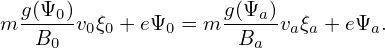(119)

Using the conservation of the kinetic energy, the above equation is written

(g(Ψ ) g(Ψ ) ) mv0 ----0ξ0 − ---a-ξa = e(Ψa − Ψ0). B0 Ba

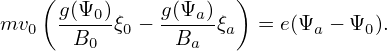(120)

Using the conservation of μ, we obtain

2 2 1−-ξa-= 1−-ξ0, Ba B0

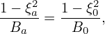(121)

which can be written

∘ ------------- ξa = ± 1− Ba-(1− ξ20). B0

(122)

where we does not distinguish between circulating particles and trapped particles. If a particle is a circulating one, then v_∥ does not change sign and thus ξ does not change sign either. In this case, equation (122) is written

∘ ------------- ξa = sign(ξ0) 1 − Ba(1 − ξ20). B0

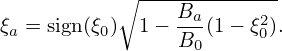(123)

If a particle is a trapped one, then both signs ± in Eq. (122) are possible.

Using Eq. (122), equation (120) is written

[ ∘ -------------] mv g(Ψ0)ξ ∓ g(Ψa) 1 − Ba(1− ξ2) = e(Ψ − Ψ ), 0 B0 0 Ba B0 0 a 0

(124)

which can be arranged in the form

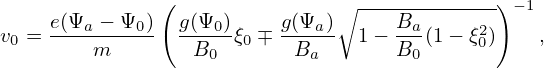e(Ψ − Ψ )( g(Ψ ) g(Ψ )∘ ----B--------) −1 v0 =---a----0- ---0-ξ0 ∓----a 1 − -a(1 − ξ20) , m B0 Ba B0

(125)

Equation (125) gives the velocity v₀ needed for the particle to reach the ﬂux surface Ψ_a. The value of v₀ given by Eq. (125) varies, depending on the value of B_a, i.e., depending on the poloidal location on the boundary magnetic ﬂux surface. By scanning the poloidal location on the boundary ﬂux surface, we can obtain the minimum value of v₀, v_{0 min}, which is the minimum velocity for a particle with the initial condition (Ψ₀,B₀,ξ₀) to reach the ﬂux surface Ψ_a.

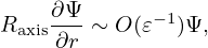
To evaluate the minimum energy for the ions to be lost, we need choose a speciﬁc magnetic conﬁguration. Next, we consider a simple large aspect ratio magnetic conﬁguration.

7.2 Large aspect ratio equilibrium

Deﬁne (r,𝜃,ϕ) coordinates by

R(r,𝜃) = Raxis + rcos𝜃,

(126)

Z(r,𝜃) = rsin 𝜃,

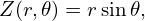(127)

where (R,ϕ,Z) are the cylindrical coordinates and R_axis is a constant. The Jacobian 𝒥 of (r,𝜃,ϕ) coordinates can be calculated using the deﬁnition, yielding 𝒥 = −Rr (refer to my notes on equilibrium).

In (r,𝜃) coordinates, the toroidal elliptic operator Δ^⋆Ψ is given by (refer to my notes on equilibrium):

2 ( ) Δ ⋆Ψ = 1-∂r ∂Ψ-+ 12 ∂-Ψ2 −----1---- ∂Ψ-cos𝜃 − ∂Ψ-1sin𝜃 . r∂r ∂r r ∂ 𝜃 R0 + rcos𝜃 ∂r ∂𝜃 r

(128)

Assume that the toroidal current density J_ϕ is given and is uniform distributed, J_ϕ = I∕S, where I is the total current within a boundary magnetic surface, S is the poloidal area enclosed by the boundary magnetic surface Since J_ϕ is given, then the expression J_ϕ = − 1
μ0R Δ^⋆Ψ can be used as a constraint for Ψ, i.e.,

1 ∂ ∂Ψ 1 ∂2Ψ 1 ( ∂Ψ ∂Ψ 1 ) I - --r---+ 2---2-− ------------ ---cos𝜃− ---- sin𝜃 = − μ0(Raxis + rcos𝜃)-, r ∂r ∂r r ∂𝜃 Raxis +r cos𝜃 ∂r ∂𝜃r S

(129)

We consider the region 𝜀 = r∕R_axis ≪ 1 (large aspect ratio regime), and further assume the following orderings

∂Ψ Raxis∂r- ∼ O(𝜀−1)Ψ,

(130)

and

∂Ψ-∼ O (𝜀0)Ψ. ∂𝜃

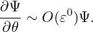(131)

Then the leading order of Eq. (129) is written as

1-∂r ∂Ψ-= − μ R I. r∂r ∂r 0 axisS

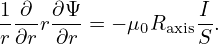(132)

One solution to the above equation is

Ψ = − μ0IRaxisr2. 4S

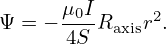(133)

In the (r,𝜃,ϕ) coordinates, the gradient of Ψ is written

∂Ψ ∂Ψ ∂Ψ ∇Ψ = -∂r ∇r + ∂𝜃-∇ 𝜃+ ∂ϕ-∇ϕ μ I = − -0-Raxisr∇r (134) 2S

Then the poloidal magnetic ﬁeld is written as

Bp = ∇ Ψ × ∇ϕ μ I = − -0-Raxisr∇r × ∇ ϕ 2S ( ) = − μ0IRaxisr − 1-∂r- . (135) 2S 𝒥 ∂𝜃

In terms of the cylindrical coordinate system (R,ϕ,Z) and its unit basis vector e_R and e_Z , a location vector r is written as

r = R(r,𝜃)eR (ϕ) + Z(r,𝜃)eZ,

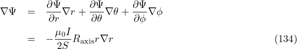
(136)

then in (r,𝜃,ϕ) coordinates, we obtain

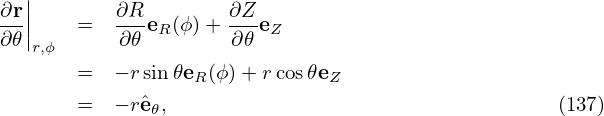
∂r || ∂R ∂Z ∂𝜃-|| = ∂𝜃-eR(ϕ)+ ∂𝜃-eZ r,ϕ = − rsin𝜃eR(ϕ)+ rcos𝜃eZ = − rˆe𝜃, (137)

where

_𝜃 = cos𝜃e_Z − sin𝜃e_R(ϕ) is a unit vector. Then Eq. (135) is written as

( ) Bp = − μ0IRaxisr −-reˆ𝜃 2S Rr μ0I------r----- = − 2S 1 + Rraxis cos𝜃ˆe𝜃 (138)

The toroidal component of the magnetic ﬁeld is written

g(Ψ-) ---g(Ψ-)---- B ϕ = R = Raxis + rcos𝜃.

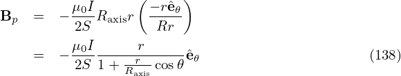
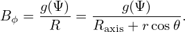(139)

Consider the case that g(Ψ) is a constant function, g(Ψ) = B_ϕ0R_axis, then Eq. (139) is written

B B ϕ =-----rϕ0---- 1 + Raxis cos𝜃

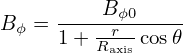(140)

I am curious about what the safety factor q looks like for the above ﬂat current density proﬁle. Let us calculate q by using q = dΨ_t∕dΨ_p.

∮ ∮ r dΨt = drBϕdℓp = drg R-d𝜃

(141)

μ0I dΨp = 4S-Raxis2rdr

(142)

Then

∮ g- ∮-1 ∮ q = dΨt-= μdrI--Rrd𝜃--= gμI-R-d𝜃-= μI-g---- ---1----d𝜃. dΨp 40S-Raxis2rdr 40S Raxis2 20S R2axis 1+ 𝜀cos𝜃

(143)

Using maxima to perform the above integral, the above expression is written as

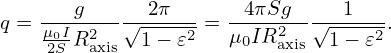q =-μ0Ig-2--√-2π---= -4πSg2--√--1---. 2S R axis 1− 𝜀2 μ0IRaxis 1− 𝜀2

(144)

pict

Figure 28: Minimum loss energy as a function of the cosine of the launching pitch angle. ρ = 0.98

———————————

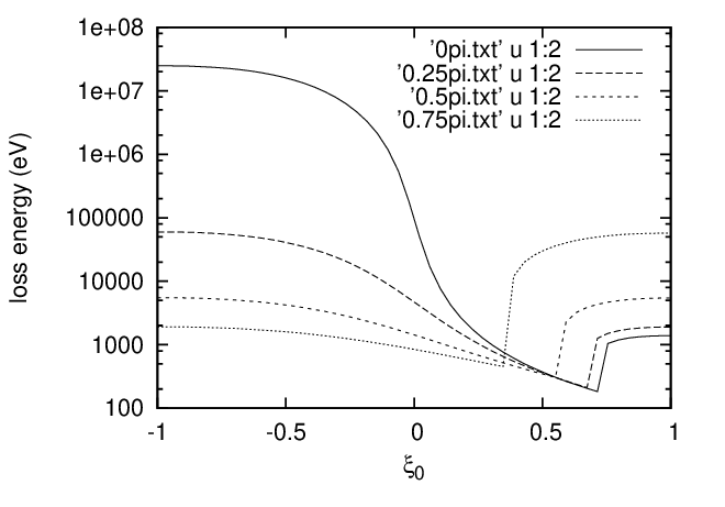
The minimum value of v₀, denoted with v_{0 min}, is reached when 𝜃 = π or 𝜃 = 0 depends on the ± in Eq. (??).

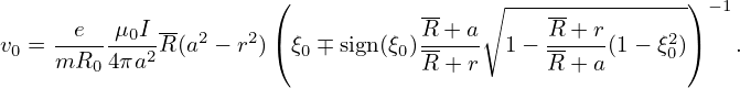( -- ∘ ---------------)− 1 v0 =--e- μ0I-R-(a2 − r2)( ξ0 ∓ sign(ξ0)R-+-a 1− R-+-r(1− ξ20)) . mR0 4πa2 R + r R + a

(145)

v0min(ξ0) = max(min(v0(ξ0,𝜃)),0)

(146)

(in practice ψ_a is usually diﬀerent from the actual poloidal ﬂux Ψ_p and is related to Ψ_p by ψ_a = ±|Ψ_p|∕2π + C, where C is a constant)

We consider the conﬁnement of the particles. The method is to determine whether the particles can reach a boundary ﬂux surface by making use of the three constants of the motion. The boundary ﬂux surface is labeled by ψ_a, where ψ_a is the poloidal ﬂux within that ﬂux surface.

[next] [prev] [prev-tail] [front] [up]