Comparison with linear theory

Next, we compare the numerical results with the electron plasma wave dispersion relation, which is given by[1]

$$1 + 2 \left( \frac{\omega_p}{k v_t} \right)^2 [1 + \zeta Z (\zeta)] = 0,$$ (83)

where $\zeta = \omega / k v_t$, and

$$Z (\zeta) = \frac{1}{\sqrt{\pi}} \int_C \frac{e^{- z^2}}{z - \zeta} d z,$$ (84)

is the plasma dispersion function. The plasma dispersion function is related to the error function of imaginary argument by

$$Z (\zeta) = i \sqrt{\pi} \exp (- \zeta^2) \ensuremath{\operatorname{erfc}} (- i \zeta) .$$ (85)

The $\ensuremath{\operatorname{erfc}}$ function is implemented in Wolfram Mathematica. By using $\ensuremath{\operatorname{FindRoot}}$ function of Wolfram Mathematica, the equation (83) can be easily solved numerically to find the root. For the parameter used in the simulation $k v_t / \omega _p = 0.5$, $\ensuremath{\operatorname{Findroot}}$ gives $\zeta = 2.4508 - i 0.0725$. From this, we obtain $\omega / \omega_p = \zeta k v_t / \omega_p = 1.2254 - i 0.0362$.

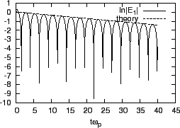
The oscillation frequency of the electric field can be estimated by counting the peaks in Fig. 8, from which we obtain $\omega_r / \omega_p = 1.226$, which agrees the theoretic value $1.2254$ given above. Figure 8 shows that the amplitude of the electric filed decreases exponentially with time. Figure 9 compares the theoretic growth rate with the simulation results, which also shows good agreement with each other.

Figure 9: Comparison of the damping rate given by Eq. (83) $(\gamma / \omega_p = - 0.0362)$ with the simulation results. $k v_t / \omega _p = 0.5$.

In the weak growth rate approximation, the real frequency of electron plasma wave is given by

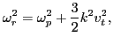$$\omega^2_r = \omega_p^2 + \frac{3}{2} k^2 v_t^2,$$ (86)

for a Maxwellian plasma. For the numerical case given here, $k v_t / \omega _p = 0.5$. Using this in Eq. (86), we obtain $\omega_r / \omega_p = 1.173$, which roughly agrees with the exact value $\omega_r / \omega_p = 1.2254$.

In the weak growth rate approximation, the growth rate is given by Eq. (45), i.e.,

$$\gamma = \frac{\pi \omega \omega_p^2}{2\vert k\vert k} \frac{1}{n_0} \left[ \frac{d f_0 (v)}{d v} \right]_{v = \omega / k},$$ (87)

Using this, we obtain

$$\gamma = \frac{\pi \omega \omega_p^2}{2 k\vert k\vert} \frac{1}{n_0} \left... ...v^2}{v_t^2} \right) \left( - \frac{2 v}{v_t^2} \right) \right]_{v = \omega / k}$$

$$= \frac{\pi \omega \omega_p^2}{2 k^2} \left[ \frac{1}{v_t \sqrt{\pi... ...omega^2}{k^2 v_t^2} \right) \left( - \frac{2 \omega}{k v_t^2} \right) \right] .$$ (88)

From this, we obtain

$$\frac{\gamma}{\omega_p} = \sqrt{\pi} \frac{\omega_p}{k v_t} \left... ...\left( - \frac{\omega^2 / \omega_p^2}{k^2 v_t^2 / \omega_p^2} \right) \right] .$$ (89)

Using $\omega / \omega_p = 1.225$ in Eq. (89), we obtain $\gamma / \omega_p = - 0.0524$, which roughly agrees with the exact value $\gamma / \omega_p = - 0.0362$ obtained above. Note that if we used $\omega \approx \omega_p$, instead of the exact frequency $\omega = 1.225 \omega_p$, then Eq. (89) would give $\gamma / \omega_p = - 0.259$, which is almost one order larger than the exact value $\gamma / \omega_p = - 0.036$. This highlights the inaccuracy of the approximate formula we encounter in textbooks[1], where $\omega = \omega_p$ is used to estimate the damping rate.