Denote the strength of the equilibrium magnetic field at the magnetic axis by
 , the mass density at the magnetic axis by
  , and the major radius
of the magnetic axis by
, and the major radius
of the magnetic axis by  . Define a characteristic speed
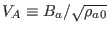 , which is the Alfvén speed at the magnetic
axis. Using the Alfvén speed, we define a characteristic frequency
, which is the Alfvén speed at the magnetic
axis. Using the Alfvén speed, we define a characteristic frequency
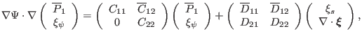
 . Multiplying the matrix equation (134)
by
. Multiplying the matrix equation (134)
by
 gives
gives
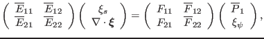 |
(154) |
with new quantities defined as follows:
![$ \overline{P}_1 \equiv P_1 / [B_a^2 /
(2{\textmu}_0)]$](img378.png) ,
,
 ,
,
 ,
,
 ,
,
 ,
,
 , and
, and
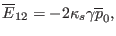
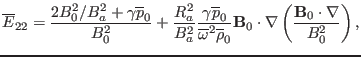
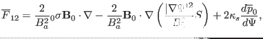
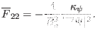
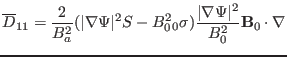
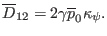
 . Using the equations (135),
(136), (140), (137), (138), and
(142), the expression of
. Using the equations (135),
(136), (140), (137), (138), and
(142), the expression of
 ,
,
 ,
,
 ,
,
 ,
,
 , and
are written respectively as
, and
are written respectively as
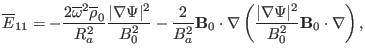 |
(155) |
 |
(156) |
 |
(157) |
 |
(158) |
 |
(159) |
 |
(160) |
where
 ,
,
 ,
,
![$ \overline{p}_0 = p_0 / [B_a^2 / (2{\textmu}_0)]$](img398.png) . Next, consider
re-normalizing the matrix equation (145). Multiply the first equation
of matrix equation (145) by
, giving
. Next, consider
re-normalizing the matrix equation (145). Multiply the first equation
of matrix equation (145) by
, giving
 |
(161) |
with the new matrix elements defined as follows:
 ,
,
 , and
, and
 . (Note that, although the second equation of
matrix equation (161) uses
. (Note that, although the second equation of
matrix equation (161) uses
 , instead of
  , as a
variable , it is actually identical with the second equation of matrix
equation (145) because the
term is multiplied by
zero.) Using Eqs. (147), (148) (149) , we obtain
, as a
variable , it is actually identical with the second equation of matrix
equation (145) because the
term is multiplied by
zero.) Using Eqs. (147), (148) (149) , we obtain
 |
(162) |
 |
(163) |
 |
(164) |
Note that, after the normalization, all the coefficients of the resulting
equations are of the order  , thus, are suitable for accurate numerical
calculation. Also note that, for typical tokamak plasmas, the normalization
factor
is of the order
, thus, are suitable for accurate numerical
calculation. Also note that, for typical tokamak plasmas, the normalization
factor
is of the order  , which is six order
away from . Therefore the normalization performed here is necessary for
accurate numerical calculation. [If the normalizing factor is two (or less)
order from , then, from my experience, it is usually not necessary to
perform additional normalization for the purpose of optimizing the numerical
accuracy, i.e., the original units system has provided a reasonable
normalization. Of course, suitable re-normalization will be of benefit to
developing a clear physical insight into the problem in question.]
, which is six order
away from . Therefore the normalization performed here is necessary for
accurate numerical calculation. [If the normalizing factor is two (or less)
order from , then, from my experience, it is usually not necessary to
perform additional normalization for the purpose of optimizing the numerical
accuracy, i.e., the original units system has provided a reasonable
normalization. Of course, suitable re-normalization will be of benefit to
developing a clear physical insight into the problem in question.]
yj
2015-09-04