Numerical results of global modes

When analyzing the modes calculated numerically, we need to distinguish two kinds of modes: the continuum modes and the gap modes. In principle, the continuum mode is defined as the mode whose frequency is within the Alfven continua while the gap mode is defined as the mode whose frequency is within the frequency gap of the Alfven continua. However, for realistic equilibria, any given frequency will touch the continua at one of the radial locations.

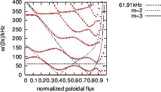
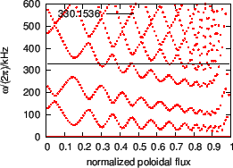
However, for realistic structure of continua, both the range and the center of the frequency of a gap change with the radial coordinate, as is shown in Fig. 16. As a result, a given frequency usually can not be within a gap for all radial locations, i.e., the frequency usually intersects the Alfven continua at some radial locations. These locations are the Alfven resonant surfaces. As is pointed out in Ref. [], the mode structure have singularity given by $[c_1 \ln \vert \psi - \psi_s \vert + c_2]$ at the resonant surface, where $\psi_s$ is the radial coordinate of the resonant surface and $c_2$ can have finite discontinuity.

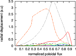
In practice, continuum modes can be easily distinguished from gap modes by examining the radial structure of the poloidal harmonics of the mode. If the radial mode structure has dominant singularities at the Alfven resonant surfaces, then the modes are continua modes. If the dominant peaks of the mode are not at the Alfven resonant surfaces, then the mode is probably a gap mode (further confirmation can be obtained by examining poloidal mode number of the dominant harmonics, discussed later). The mode structure of gap modes can also have singular peak at the resonant surface, but the peak is usually smaller than the dominant peak.

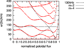
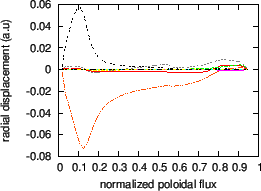
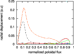
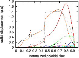
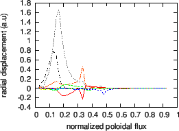
Mode structure of a $n = 1$ TAE mode is plotted in Fig. 20

Figure 20: Real part (a), imaginary part (b), and amplitude (c) of the poloidal harmonics of a $n = 1$ TAE mode as a function of the radial coordinate. The frequency of the mode is $f = 101 \ensuremath {\operatorname {kHz}}$. The poloidal harmonics with $m = 1$ and $m = 2$ are dominant. The equilibrium used for this calculation is for EAST shot 38300 at 3.9s (G-file name: g038300.03900). (D)

Figure 21: Slow sound approximation of the continua. Also plotted are the frequency of the TAE mode ( $f = 101 \ensuremath {\operatorname {kHz}}$) and the $m = 1$ and $m = 2$ continua in cylindrical limit. Toroidal mode number $n = 1$. The equilibrium is the same as Fig (D)

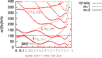
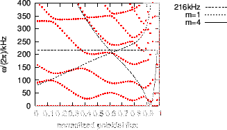
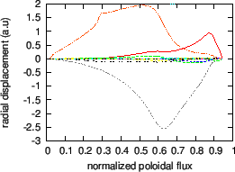
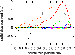
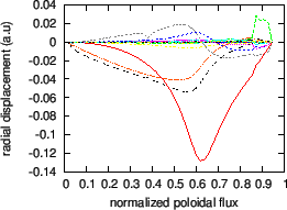
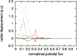
Fig. 22. plots the radial mode structure of another TAE with frequency $f = 61.91 \ensuremath {\operatorname {kHz}}$.

Figure 22: Real part (a), imaginary part (b), and amplitude (c) of the poloidal harmonics of a $n = 1$ TAE mode as a function of the radial coordinate. The frequency of the mode is $f = 61.91 \ensuremath {\operatorname {kHz}}$. The poloidal harmonics with $m = 2$ and $m = 3$ are dominant. The equilibrium used for this calculation is for EAST shot 38300 at 3.9s (G-file name: g038300.03900). (D)

Figure 23: Slow sound approximation of the continua. Also plotted are the frequency of the TAE mode ( $f = 61.91 \ensuremath {\operatorname {kHz}}$) and the $m = 2$ and $m = 3$ continua in cylindrical limit. Toroidal mode number $n = 1$. The equilibrium is the same as Fig (D)

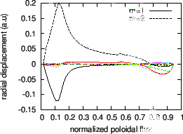
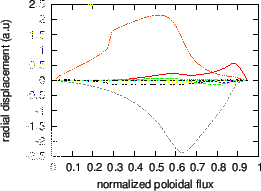
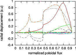
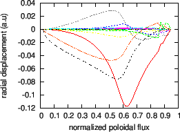
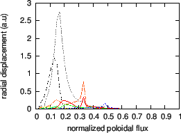
An example of ellipticity-induced Alfven Eigenmode (EAE) is plotted in Fig. 24. The mode is identified as an EAE mode because it satisfies the following three requirements: (1) the mode has two dominant harmonics with poloidal mode number differing by two ($m = 2$ and $m = 4$ for this case); (2) the frequency of the mode $f = 130 \ensuremath {\operatorname {kHz}}$ is within in the continuum gap formed due to the coupling of these two poloidal harmonics; (3) the location of the peak of the radial mode structure is within the continuum gap.

Figure 24: Real part (a), imaginary part (b), and amplitude (c) of the poloidal harmonics of a $n = 1$ EAE mode as a function of the radial coordinate. The poloidal harmonics with $m = 2$ and $m = 4$ are dominant. $f = 130 \ensuremath {\operatorname {kHz}}$. The equilibrium is for EAST shot 38300 at 3.9s (G-file name: g038300.03900). (D)

Figure 25: $n = 1$ Alfvén continua (D)

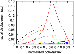
An example of non-circularity-induced Alfven Eigenmode (NAE) is plotted in Fig. 26.

Figure 26: Real part (a), imaginary part (b), and amplitude (c) of the poloidal harmonics of a $n = 1$ NAE mode as a function of the radial coordinate. The poloidal harmonics with $m = 1$ and $m = 4$ are dominant. The frequency of the mode is $f = 216 \ensuremath {\operatorname {kHz}}$. The equilibrium is for EAST shot 38300 at 3.9s (G-file name: g038300.03900). (D)

Figure 27: $n = 1$ Alfvén continua (D)

$n = 4$

Figure 28: Real part (a), imaginary part (b), and amplitude (c) of the poloidal harmonics of a $n = 4$ EAE mode as a function of the radial coordinate. The frequency of the mode is $f = 330 \ensuremath {\operatorname {kHz}}$. The poloidal harmonics with $m = 5$ and $m = 7$ are dominant. The poloidal harmonics are truncated into the range $m = [- 10, 10]$ in the numerical calculation. The equilibrium is for EAST shot 38300 at 3.9s (G-file name: g038300.03900). (H)

Figure 29: The frequency of the EAE mode given in Fig. 28. (H)