A plasma can be considered to be composed of a set of classical point particles, with motion subject to Newton’s equations and with the Lorentz forces and electromagnetic field derived from Maxwell’s equations. Because of the huge number of particles in a plasma, the above microscopic representation is intractable, and simplifications must be sought[8].
A usual procedure is to approximate the set of particles by a continuum distribution function. This step involves some kind of averaging procedure to remove certain spatial and temporal frequencies that are associated with the graininess of the particle description (particle corelations, i.e., collisions). It is important to note that approximation is introduced in passing from the microscopic particle representation to the continuum distribution function.
The averaging procedure involves a small parameter, the so-called “plasma parameter,” which is the inverse of the number of particles contained in a Debye sphere. The collisionless Boltzmann equation, also known as the Vlasov equation, emerges from the averaging procedure as the approximation at zero order in the plasma parameter. What is discarded in the the zeroth order approximation is the so-called collisional effects. In the first order approximation, there appear additional terms, which is a representation of the Coulomb collision effects.
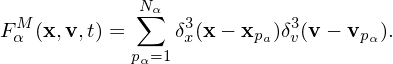
The discrete microscopic distribution function (Klimontovich-Dupree distribution function) (Chapter 3 in Nicholson (1983)) is written as
|
| (149) |
Then the partial time derivative of FαM is written as
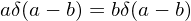
Using the property of the Dirac delta function:
 | (152) |
expression (151) is written as
![∂FαM(x,v,t) ∑Nα 3 3 ∑Nα 3 qα- M M 3
∂t = − δv(v − vpα)v⋅∇x [δx(x− xpa)]− δx(x − xpa)mα [E (x)+ v × B (x)]⋅∇vδv(v− vpα)
pα=1 pα=1
∑Nα 3 3 qα- M M ∑Nα 3 3
= − v⋅∇x δv(v − vpα)[δx(x− xpa)]− m α[E (x )+ v× B (x)]⋅∇v δx(x − xpa)δv(v − vpα )
pα=1 pα=1
= − v⋅FαM − qα-[EM (x) +v × BM (x)]⋅∇vF Mα , (153)
mα](particle_simulation177x.png)
![M
∂Fα-(x,v,t)-+ v⋅FαM + qα-[EM (x) + v× BM (x)]⋅∇vF Mα = 0
∂t m α](particle_simulation178x.png) | (154) |
This is the Klimontovich equation of the microscopic distribution function.
Note that Boltzmann equation provide a mesoscopic rather than a microscopic description because of the spatio-temporal averaging involved in deriving the Boltzmann equation
The particle-in-cell (PIC) method has obvious structural similarities to a direct simulation of the microscopic model of the plasma outlined above, but this is essentially misleading: Particle-in-cell simulation should be understood to be a Monte Carlo solution of the Boltzmann equation (or the Vlasov equation), i.e., the PIC method is solving a continuum mesoscopic kinetic equation rather than the primitive microscopic model of a plasma.
two things that reduce collision: (1) finite-size particle used in doing the deposition and force iterpolation and (2) finite grid size used in solving the field equation.
The nearest grid point deposition and force interpolation correspond zero sized particle, i.e., delta function
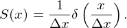 | (155) |
![M Nα Nα
∂Fα-(x,v,t) = ∑ δ3(v− vp ) ∂-δ3(x− xp )+ ∑ δ3(x− xp ) ∂-δ3(v − vp ) (150)
∂t pα=1 v α ∂t x a pα=1 x a ∂t v α
Nα Nα
= − ∑ δ3(v − vp )∂xpα-⋅∇x[δ3(x − xp )]− ∑ δ3(x− xp )∂vpα-⋅∇vδ3(v− vp )
pα=1 v α ∂t x a pα=1 x a ∂t v α
Nα N α
= − ∑ δ3(v − v )v ⋅∇ [δ3(x− x )]− ∑ δ3(x − x )-qα[EM (x )+ v × BM (x )]⋅∇ δ3(v −(v151))
pα=1 v pα pα x x pa pα=1 x pam α pα pα pα v v pα](particle_simulation175x.png)