5.12 Integration of orbit and weight of markers

The evolution equation of orbit and weight can be generally written as

(118)

(119)

where H₁ and H₂ are known function. Note that E, as well as r and v, depends on time t. However E is not specified as an evolution equation. Instead, E is determined by a field equation, namely Poisson’s equation.

The classical 4th Runge-Kutta time integrator requires four evaluations of the function appearing on the right-hand side of the equation of motion per time step. In PIC method, this corresponds to that the field equation needs to be solved for four times. For large-scale simulation (e.g. spatial three-dimension simulation), solving the field equation is usually time-consuming. Considering this, lower order Runge-Kutta (e.g. 2nd order), which requires fewer times of evaluation of functions (and thus fewer times of solving the field equation) may be preferred in practice.

We use the 2nd Runge-Kutta method to integrate orbit and weight of markers. In this method, r, v, and w are first integrated from t_n to the half time-step t_n+1∕2 using (r_n,v_n,E_n) to evaluate the right-hand side of Eqs. (118) and (119). Then we solve the Poisson’s equation at t_n+1∕2 to obtain E_n+1∕2 using the already obtained values of (r_n+1∕2,v_n+1∕2,w_n+1∕2). After E_n+1∕2 is obtained, r, v, and w are integrated from t_n to t_n+1 by using the values at the half time-step, namely (r_n+1∕2,v_n+1∕2,w_n+1∕2,E_n+1∕2). Forgetting to solve the field equation at t_n+1∕2 to get E_n+1∕2 is one of the mistakes I made during writing the code. Forgetting to do this means that I am still using E_n, instead of E_n+1∕2, in taking the full step from t_n to t_n+1, which amounts to the (inaccurate and thus may be unstable) Euler scheme.

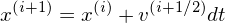
[Besides, the leapfrog scheme (2nd order accuracy) is often adopted to integrate the equations of motion. This scheme is given by

(120)

(121)

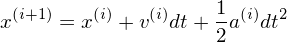
where a_i = a_i(x_i) is the acceleration of the particle at the time step i. The leapfrog scheme given by Eqs. (121) and (120) can be equivalently written as[6]

(122)

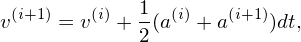(123)

The leapfrog scheme given by Eqs. (122) and (123) was implemented in my code, but was not tested seriously (I usually used the 2n Runge-Kutta method discussed above). Note  that, for electrostatic case, a⁽ⁱ⁺¹⁾ is independent of v⁽ⁱ⁺¹⁾ and depends only on x⁽ⁱ⁺¹⁾, which is already obtained by Eq. (122). Thus the scheme given by Eqs. (122) and (123) is still an explicit scheme.]