Free boundary equilibrium problem

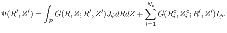
Free boundary equilibrium problem refers to the case where the value of $\Psi$ on the boundary of the computational box is unknown and must be determined from the current from both the plasma and external coils. Suppose the computational box is a rectangle on $(R, Z)$ plane. If all the current perpendicular to $(R, Z)$ plane is known, the value of $\Psi$ at any point can be uniquely determined by using the Green function method, which gives

$$\Psi (R', Z') = \int_P G (R, Z ; R', Z') J_{\phi} d R d Z + \sum_{i = 1}^{N_c} G (R^c_i, Z_i^c ; R', Z') I_{\phi} .$$ (98)

In solving the equilibrium problem, the current in external coils is given and known while the current carried by the plasma is unknown, which need to be derived from the information of $\Psi$ via Eq. (61), i.e.,

$$J_{\phi} = - \frac{1}{\mu_0 R} \triangle^{\ast} \Psi .$$ (99)

To numerically solve GS equation within the computational box, we need the value of $\Psi$ on the boundary of the box as a boundary condition. Thus we need to adopt some initial guess of the value of $\Psi$ on the boundary, then solve the GS equation to get the value of $\Psi$ within the computational box. Using the computed $\Psi$, we can calculate the value of the plasma current perpendicular to the $(R, Z)$ plane through Eq. (99). After this, all the current (current in the plasma and in the external coils) perpendicular to the poloidal plane is known, we can calculate the value of $\Psi$ on the boundary of the box, $\Psi_b$, by using the Green function formulation Eq. (98). Note that $\Psi_b$ calculated this way usually differs from the initial guess of the value of $\Psi$ on the boundary. Thus, we need to use the $\Psi_b$ calculated this way as a new guess value of $\Psi$ on the computational boundary and repeat the above procedures. The process is repeated until $\Psi_b$ obtained in two successive iterations agrees with each other to a prescribed tolerance.

Before considering the free boundary equilibrium problem, it is instructive to consider the fixed boundary equilibrium problem, where the shape of the last closed flux surface is given, because this kind of problem provides basic knowledge for dealing with the more complicated free boundary problem. In dealing with the fixed boundary problem, the curvilinear coordinate system is useful. Specifically, the convenience provided by a curvilinear coordinate system in solving the fixed boundary tokamak equilibrium problem is that the curvilinear coordinates can be properly chosen to make one of the coordinate surfaces coincide with the given boundary flux surface, so that the boundary condition becomes trivial in this curvilinear coordinate system.

Next section discusses the basic theory of curvilinear coordinates system. (I learned the theory of general coordinates from the appendix of Ref. [3], which is concise and easy to understand.) Many analytical theories and numerical codes use the curvilinear coordinate systems that are constructed with one coordinate surface coinciding with the magnetic surface. These kinds of curvilinear coordinates are usually called the magnetic surface coordinates. In these coordinate systems, we need to choose a poloidal coordinate $\theta$ and a toroidal coordinate $\zeta$. A particular choice for $\theta$ and $\zeta$ is such one that makes the magnetic field lines be straight lines on $(\theta, \zeta)$ plane. This kind of coordinate system is usually called a flux coordinate system.