A Efficient method of computing DFT: Fast Fourier Transformation (FFT) algorithm (not finished)

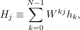
The DFT is defined by Eq. (34), i.e.,

(82)

where W = exp(2πi∕N). Equations (82) indicates that the DFT is the multiplication of a transformation matrix M_kj ≡ W^kj with a column vector h_k, where the transformation matrix M_kj is symmetric and called DFT matrix. In the matrix form, the DFT is written as

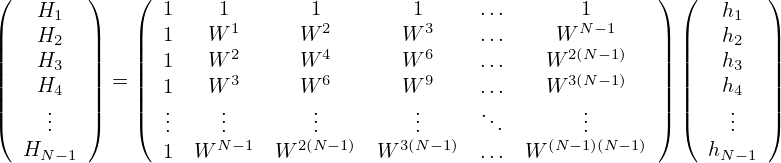(83)

If directly using the definition in Eq. (83) to compute DFT, then a matrix multiplication need to be performed, which requires O(N²) operations. Here the powers of W are assumed to be pre-computed, and we define “an operation” as a multiplication followed by an addition.

The Fast Fourier Transformation (FFT) algorithm manage to reduce the complexity of computing the DFT from O(N²) to O(N log ₂N) by factoring the DFT matrix M_kj into a product of sparse matrices.

The original paper on FFT is Cooley and Tukey’s paper: An algorithm for the machine calculation of complex Fourier series, which turns out to be a very concise paper.

Suppose N is a composite, i.e., N = r₁ ⋅ r₂. Then the indices in Eq. (82) can be expressed as

(84)

(85)

Then, one can write

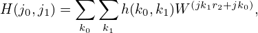(86)

Noting that

(87)

Eq. () is written as

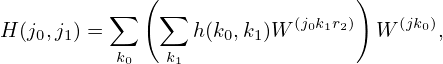(88)

where the inner sum over k₁ is independent of j₁ and can be defined as a new array

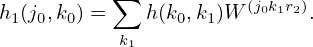(89)

Then

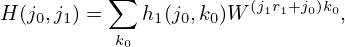(90)

There are N elements in the array h₁, each requiring r₁ operations, giving a total of Nr₁ operation to obtain h₁. Similarly, it takes Nr₂ operations to calculate H from h₁. Therefore, this two-step algorithm requires a total of N(r₁ + r₂) operations.