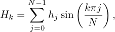
There are several slightly different types of Discrete Sine Transforms (DST). One form I saw in W. Press’s numerical recipe book is given by
|
| (55) |
where h0 = hN = 0 are assumed. This form can be obtained by replacing DFT’s exponential function exp(2πikj∕N) by sin(πkj∕N). The inverse sine transformation is given by (I did not derive this, but had numerically verified that this transform recovers the original data if applied after the sine transform (55) (code at /home/yj/project_new/test_space/sine_expansion/t2.f90))
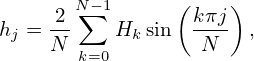 | (56) |
which is identical with the forward sine transformation except for the normalization factor 2∕N. (The terms of index 0 in both Eq. () and () can be dropped since they are zero. They are kept to make the representation look more similar to the DFT, where the index begin from zero.) Replacing j∕N in Eq. (56) by (x − x0)∕L , we obtain the reconstructing function
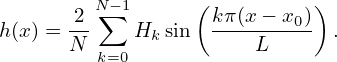 | (57) |
We need a fast method for computing the above DST. All fast methods finally need to make use of the fast method used in the computation of DFT, i.e., FFT. To make use of FFT, we need to define the DST in a way that the DST can be easily connected to the DFT so that FFT can be easily applied. A standard way of making this easy is to define the DST via the DFT of an odd extension of the original data. Next, let us discuss this.