2.3 Numerical computation of Fourier expansion coefficient

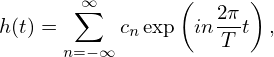
For a periodic function h(t) with a period of T, its Fourier expansion is given by

(31)

with the coefficient c_n given by

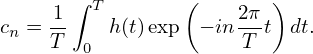(32)

How to numerically compute the Fourier expansion coefficients? A simple way is to use the rectangle formula to approximate the integration in Eq. (32), i.e.,

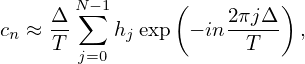(33)

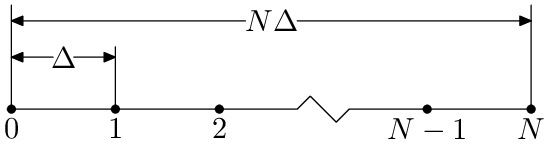
where h_j = h(t_j) and t_j = jΔ with j = 0,1,2,…,N − 1 and Δ = T∕N, as is shown in Fig. 1.

Note Eq. (33) is an approximation, which will become exact if Δ → 0. In practice, we can sample h(t) only with a nonzero Δ. Therefore Eq. (33) is usually an approximation. Do we have some rules to choose a suitable Δ so that Eq. (33) can become a good approximation or even an exact relation? This important question is answered by the sampling theorem (will be discussed in Append. B), which sates that a suitable Δ to make Eq. (33) exact is given by Δ ≤ 1∕(2f_c), where f_c = N_c∕T is the largest frequency contained in h(t) (i.e, c_n is zero for |n|≥ N_c).

f_s ≡ 1∕Δ is called sampling frequency. Then the above condition can be rephrased as: the sampling frequency should be larger than 2f_c.