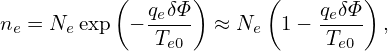
Assume that the total electron density satisfies the Boltzmann distribution on each magnetic surface, i.e.,
| (297) |
where Ne is a radial function. Note that this does not imply that the equilibrium density is Ne (it just implies that the total density is Ne at the location where δΦ = 0, which can still be different from the equilibrium density).
Further assume that the magnetic surface average of electron density perturbation (δne = ne −ne0) is zero, i.e.,
| (298) |
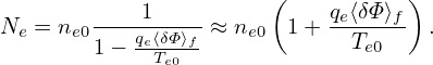
where ne0 is the equilibrium electron density, ⟨…⟩f is the magntic surface averaging operator. Using Eq. (297) in the above condition, we get
| (299) |
Then expression (297) is written as
| (300) |
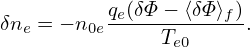
Then the perturbation δne = ne − ne0 is written as
| (301) |
This model for electron response is often called adiabatic electron.
Pluging expression (301) into the Poisson equation (231), we get
| (302) |
When solving the Poisson equation, the equation is Fourier expanded into toroidal harmonics. Each harmonic is independent of each other, so that they can be solved independently. For n≠0 harmonics, the ⟨δΦ⟩f terms is zero and thus the the electron term is easy to handle because it’s a local response. There is some difficulty in solving the n = 0 harmonic because the ⟨δΦ⟩f term is nonzero.
I use the following method to obtain ⟨δΦ⟩f.
First slove the n = 0 harmonic of the following equation:
| (303) |
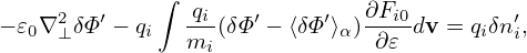
(i.e., Eq. (302) with the electron contribution dropped). Let δΦ′ denote the solution to this equation. Then it can be proved that ⟨δΦ′⟩f is equal to ⟨δΦ⟩f. [Proof:
Taking the flux surface average of Eq. (302), we obtain
| (304) |
where the adiabatic response disappears. to be continued.
]
Then solving Eq. (302) becomes easier because ⟨δΦ⟩f term is known and can be moved to the right-hand side as a source term.