5.1 Numerically testing orbit types

In the above, we plot boundary curves in the phase space (Pϕ,Λ) and get some rough ideas about possible orbits in different regions of (Pϕ,Λ) plane. Next, let us numerically examine the orbits and confirm which regions are cooresponding to passing/trapped/confined/lost regions.


pict

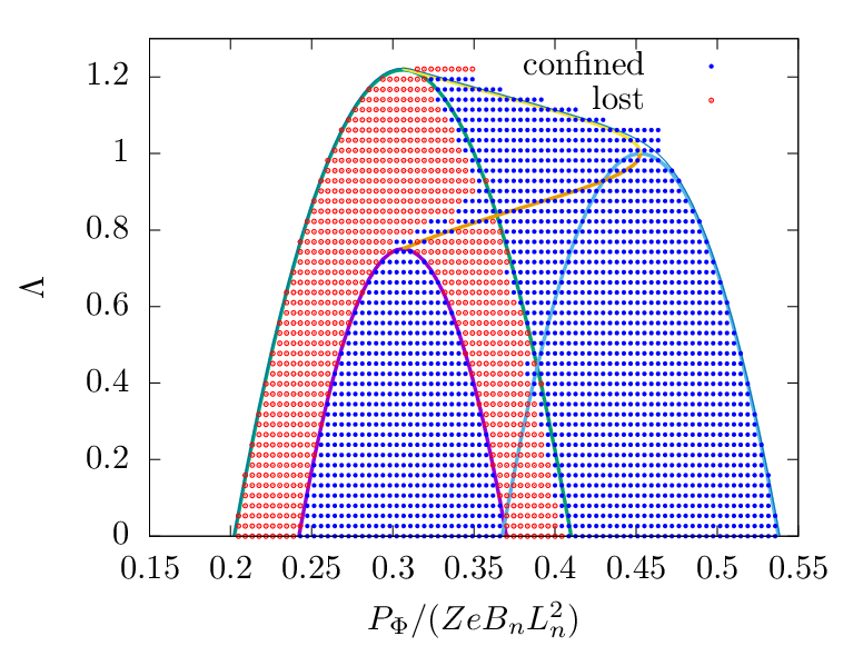
Figure 11: For E = 50keV, EAST#52340. Orbits are numerically computed to check whether they are confined (not touch the LCFS) or lost (touch the LCFS). Some particles in the loss region are numerically determined to be confined. Whether this is due to numerical errors is unclear.


pict

Figure 12: For E = 50keV, EAST#52340. Orbits are numerically computed to check whether they are passing or trapped. Some particles in the trapped region are numerically determined to be passing. Whether this is due to numerical errors is unclear.

P- =  --Pϕ----
  ϕ   ZeBnL2n
(71)

BBaxis
-g2--- 1
2m𝜀-(Pϕ ZeΨ)2

− BBaxis-1--(Pϕ − ZeΨ )2
    g2- 2m 𝜀
    BBaxis-m--- 2      2 --   --2
= −   g2  2m2 𝜀Ln(ZeBn )(Pϕ − Ψ)
    ---           --   --
= − BBax2ism-L2nΩ2n(Pϕ − Ψ)2
    --g   2𝜀
= − BBaxism-L2 (2π-)2(P- − Ψ)2
      g2  2𝜀  n T2n    ϕ
    BBaxism        --   --
= − --g2--2𝜀v2n(2π)2(P ϕ − Ψ )2
    ---
= − BBaxis-1(2π)2(P-ϕ − Ψ-)2
      g2  2𝜀
  g
m --v∥ = Pϕ − ZeΨ,
  B
(72)

     v    BZeB  L2 --   --
v∥ = -∥ = ----Lnn-n-(P ϕ − Ψ ).
     vn     mg Tn
(73)

     --
-    BΩnTn----   --
v∥ =   g   (Pϕ − Ψ)
(74)

-    B-|Z|2π --   --
v∥ = --Zg---(Pϕ − Ψ)
(75)