Averaging over initial spatial location and velocity of particles

Assume the distribution function of the particles is given by $F (v_0, z_0) = f (v_0) h (z_0)$ and $h (z_0) = 1$, i.e. the distribution is uniform in space.

Consider the averaging over the initial position of particles. Define

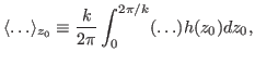$$\langle \ldots \rangle_{z_0} \equiv \frac{k}{2 \pi} \int_0^{2 \pi / k} (\ldots) h (z_0) d z_0,$$ (25)

which is an operator averaging over the initial position of particles in the interval of one wave length. Using this operator on both sides of Eq. (24), we obtain

$$\left\langle \frac{d}{d t} \left( \frac{1}{2} m v^2 \right) \right\rangle_{z_0} = \langle v_0 q E \cos (k z_0 + \alpha t) \rangle - \left\langle \s... ...k z_0 + \alpha t) - \sin (k z_0)}{\alpha} \cos (k z_0 + \alpha t) \right\rangle$$ (26)

$$= 0 - \frac{k}{2 \pi} k v_0 \frac{(q E)^2}{m} \int_0^{2 \pi / k} \s... ...\sin (k z_0 + \alpha t) - \sin (k z_0)}{\alpha} \cos (k z_0 + \alpha t) d z_0 .$$ (27)

Note that the term $v_0 q E \cos (k z_0 + \alpha t)$ corresponds to the power of the electric field acting on those particles that move at a constant speed $v_0$. Also note this term is reduced to zero when averaged over the initial position $z_0$ no mater whether it is a resonant particle (i.e., $\alpha \approx 0$) or not (i.e., $\alpha \neq 0$). (This important fact is seldom mentioned in textbooks, which is one of the motivations that I wrote this note.) Changing to the new variable $x \equiv k z_0 + \alpha t$, the above equation is written as

$$\left\langle \frac{d}{d t} \left( \frac{1}{2} m v^2 \right) \right\rangle_{z_0} = - \frac{k}{2 \pi} k v_0 \frac{(q E)^2}{m} \int_{\alpha t}^{2 \pi ... ...alpha t} \frac{\sin (x) - \sin (x - \alpha t)}{\alpha} \cos (x) \frac{1}{k} d x$$

$$= - \frac{1}{2 \pi} k v_0 \frac{(q E)^2}{m} \int_{\alpha t}^{2 \pi ... ...t_{\alpha t}^{2 \pi + \alpha t} \frac{\sin (x - \alpha t)}{\alpha} \cos (x) d x$$

$$= - \frac{1}{2 \pi} k v_0 \frac{(q E)^2}{m} \left[ \frac{1}{\alpha^... ...{1}{\alpha} \int_{\alpha t}^{2 \pi + \alpha t} \sin (x - \alpha t) \cos (x) d x$$

$$= - \frac{1}{2 \pi} k v_0 \frac{(q E)^2}{m} \left[ \frac{\pi}{\alph... ...right] + \frac{1}{2 \pi} \frac{(q E)^2}{m} \frac{1}{\alpha} \pi \sin (\alpha t)$$

$$= \frac{(q E)^2}{2 m} \left[ - k v_0 \frac{1}{\alpha^2} \sin (\alph... ...v_0 \frac{t}{\alpha} \cos (\alpha t) + \frac{1}{\alpha} \sin (\alpha t) \right]$$

$$= \frac{(q E)^2}{2 m} \left[ - (\alpha + \omega) \frac{1}{\alpha^2}... ...ga) \frac{t}{\alpha} \cos (\alpha t) + \frac{1}{\alpha} \sin (\alpha t) \right]$$ (28)

$$= \frac{(q E)^2}{2 m} \left[ - \frac{\omega}{\alpha^2} \sin (\alpha t) + t \cos (\alpha t) + \frac{\omega t}{\alpha} \cos (\alpha t) \right],$$ (29)

which agrees with Eq. (8) in Chapter 8 of Stix's book. Next, we will average Eq. (29) over the distribution of initial velocity. Define the averaging operator in velocity space

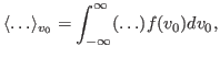$$\langle \ldots \rangle_{v_0} = \int_{- \infty}^{\infty} (\ldots) f (v_0) d v_0,$$ (30)

where $f (v_0)$ is the one-dimensional distribution function, which satisfies the following normalizing condition

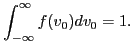$$\int_{- \infty}^{\infty} f (v_0) d v_0 = 1.$$ (31)

Changing to the variables $\alpha \equiv k v_0 - \omega$, equation (30) is written as

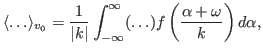$$\langle \ldots \rangle_{v_0} = \frac{1}{\vert k\vert} \int_{- \infty}^{\infty} (\ldots) f \left( \frac{\alpha + \omega}{k} \right) d \alpha,$$ (32)

Define

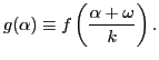$$g (\alpha) \equiv f \left( \frac{\alpha + \omega}{k} \right) .$$ (33)

then equation (32) is written as

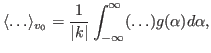$$\langle \ldots \rangle_{v_0} = \frac{1}{\vert k\vert} \int_{- \infty}^{\infty} (\ldots) g (\alpha) d \alpha,$$ (34)

Taking the average over the initial velocity, Eq. (29) is written as

$$\left\langle \left\langle \frac{d}{d t} \left( \frac{1}{2} m v^2 \right) \right\rangle_{z_0} \right\rangle_{v_0} = \left\langle \frac{(q E)^2}{2 m} \left[ - \frac{\omega}{\alpha^2}... ...\alpha t) + \frac{\omega t}{\alpha} \cos (\alpha t) \right] \right\rangle_{v_0}$$

$$= \frac{1}{\vert k\vert} \frac{(q E)^2}{2 m} \int_{- \infty}^{\inft... ...\alpha t) + \frac{\omega t}{\alpha} \cos (\alpha t) \right] g (\alpha) d \alpha$$ (35)

It can be proved that the integration $\int_{- \infty}^{\infty} t \cos (\alpha t) g (\alpha) d \alpha$ and $\int_{- \infty}^{\infty} \frac{t}{\alpha} \cos (\alpha t) g (\alpha) d \alpha$ in the above equation approach zero rapidly for large $t$ (refer to Sec. 2.5.3). Thus, in the sense of time asymptotic, we are left with only the integration of the first term, which is written as

$$- \frac{1}{\vert k\vert} \frac{(q E)^2}{2 m} \int_{- \infty}^{\infty} \frac{\omega}{\alpha^2} \sin (\alpha t) g (\alpha) d \alpha .$$ (36)