In the cylindrical geometry, continua with different poloidal mode numbers
will intersect each other, as shown in Fig. 1. Next, we calculate
the radial location of the intersecting point of two continua with poloidal
mode number  and
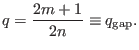
and  , respectively. In the intersecting point, we have
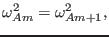 |
(237) |
i.e.
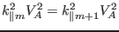 |
(238) |
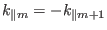
which gives
 |
(239) |
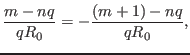
or
 |
(240) |
Inspecting the expression for
 in Eq. (323), we know
that only the case in Eq. (240) is possible, which gives
in Eq. (323), we know
that only the case in Eq. (240) is possible, which gives
 |
(241) |
which further reduces to
 |
(242) |
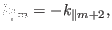
The above equation determines the radial location where the continuum
intersect the continuum. Note that a mode with two poloidal modes has
two corresponding resonant surfaces. For the case where the mode has and
poloidal harmonics, the resonant surfaces are respectively  and
and
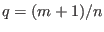 . Note that the value of
  given in Eq. (242)
is between the above two values.
given in Eq. (242)
is between the above two values.
In toroidal geometry, the different poloidal modes are coupled, and the
continuum will ``reconnect'' to form a gap in the vicinity of the original
intersecting point, as shown in Fig. . Therefore the original intersecting
point, Eq. (242), gives the approximate location of the gap.
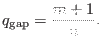
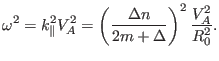
Furthermore, using Eq. (242), we can determine the frequency of the
intersecting point, which is given by
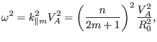 |
(243) |
which can be further written
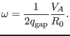 |
(244) |
According to the same reasoning given in the above, Eq. (244) is an
approximation to the center frequency of the TAE gap. The frequency and the
location given above are also an approximation to the frequency and location
of the TAE modes that lie in the gap.
For the ellipticity-induced gap (EAE gap), which is formed due to the coupling
of and  harmonics, the location is approximately determined by
 |
(245) |
which gives
 |
(246) |
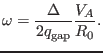
and the approximate center angular frequency is
 |
(247) |
which can be written as
Generally, for the gap formed due to the coupling of and
 harmonics, we have
which gives
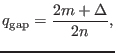 |
(248) |
and
 |
(249) |
Equation (249) can also be written as
 |
(250) |
yj
2015-09-04
