Introduction

1 Introduction

1.1 Gyrokinetic?

Electromagnetic perturbations of frequency lower than the ion cyclotron frequency are widely believed to be more important than high-frequency ones in transporting plasma in tokamaks. (This assumption can be veriﬁed numerically when we are able to do a full simulation including both low-frequency and high-frequency perturbations. This kind of veriﬁcation is not possible at present due to computation costs.)

If we assume that only low-frequency perturbations are present, the Vlasov equation can be simpliﬁed. Speciﬁcally, symmetry of the particle distribution function in the phase space can be established if we choose suitable phase-space coordinates and split the distribution function in a proper way. The symmetry is along the so-called gyro-angle α in the guiding-center coordinates (X,μ,𝜀,α). In obtaining the equation for the gyro-angle independent part of the distribution function, we need to average the equation over the gyro-angle α and thus this model is called “gyrokinetic”.

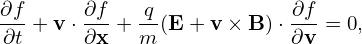
In deriving the gyrokinetic equation, the perturbed electromagnetic ﬁeld is assumed to be known and of low-frequency. To do a kinetic simulation, we need to solve the ﬁeld equation to obtain the perturbed electromagnetic ﬁeld. It is still possible that high frequency modes (e.g., compressional Alfven waves and Ω_H modes) appear in a gyrokinetic simulation. If the amplitude of high frequency modes is large, then the simulation is invalid since the gyrokinetic model is invalid in this case.

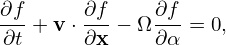
Our starting point is the Vlasov equation in terms of particle coordinates (x,v):

∂f ∂f q ∂f ∂t-+ v ⋅∂x-+ m-(E+ v × B) ⋅∂v-= 0,

(1)

where f = f(t,x,v) is the particle distribution function, x and v are the location and velocity of particles. The distribution function f depends on 6 phase-space variables (x,v), besides the time t.

1.2 Guiding-center coordinates: a simple example

Choose Cartesian coordinates (x,y,z) for the conﬁguration space x. Consider a simple case where the electromagnetic ﬁeld is a time-independent ﬁeld given by B = B₀(x,y,z) and E = 0. Let us examine the Vlasov equation in this case and look whether there is any coordinate system that can simplify the Vlasov equation.

Describe the velocity space using a right-handed cylindrical coordinates (v_⊥,α,v_∥), where v_∥ = v ⋅ e_∥, e_∥ = e_z is the unit vector along the magnetic ﬁeld, α is the azimuthal angle of the perpendicular velocity (v_⊥ = v −v_∥e_z) relative to e_x. Note that these coordinates are deﬁned relative to the local magnetic ﬁeld, which may vary in space.

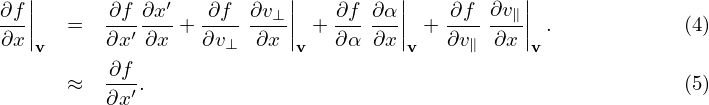
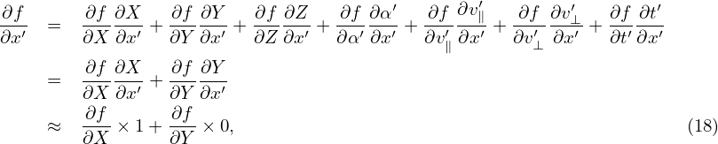
Next, let us express the spatial gradient of f in terms of partial derivatives:

∂f-|| ∂f-|| ∂f-|| ∂f|| ∂x || = ∂x || ex + ∂y || ey + ∂z|| ez. (2) v v v v

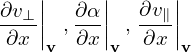
Note that this gradient is taking by holding v constant (i.e., (v_x,v_y,v_z) constant rather than (v_⊥,α,v_∥) constant). So, we need do the following coordinate transform:

( ∘ ------- ) (x,y,z,v,v ,v ) ⇒ x′ = x,y′ = y,z′ = z,v = v2+ v2,α = atan 2(v,v ),v = v x y z ⊥ x y y x ∥ z

(3)

Using chain rule, expression (2) is written as

∂f|| ∂f ∂x′ ∂f ∂v⊥ || ∂f ∂α|| ∂f ∂v∥|| ∂x|| = ∂x-′∂x-+ ∂v---∂x-|| + ∂α- ∂x|| + ∂v- -∂x|| . (4) v ⊥ v v ∥ v ≈ -∂f. (5) ∂x ′

Note that the partial derivatives

∂v || ∂α || ∂v || --⊥-|| ,---||, --∥|| ∂x v ∂x v ∂x v

(6)

are generally nonzero since the deﬁntion of (v_⊥,α,v_∥) depends on the local magnetic ﬁeld direction. In our simple case, they are zero since the magnetic ﬁeld direction is uniform. Similarly, we obtain

∂f|| ∂f --|| ≈ --′ ∂y v ∂y

(7)

∂f|| ∂f --|| = --′ ∂z v ∂z

(8)

Then, in (x′,y′,z′,v_⊥,α,v_∥) coordinates, the spatial gradient of f is written as

∂f || ∂f ∂f ∂f ---|| ≈ --′ex + --′ey +--′ez. ∂x v ∂x ∂y ∂z

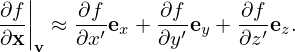(9)

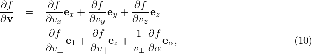
Next, consider the gradient in velocity space

∂f ∂f ∂f ∂f ∂v- = ∂v-ex + ∂v-ey + ∂v-ez x y z = ∂f-e1 + ∂f-ez +-1-∂f-eα, (10) ∂v⊥ ∂v∥ v⊥ ∂α

where e₁ = v_⊥∕|v_⊥|, v_⊥ = v − (v ⋅e_z)e_z, and e_α = e_z ×e₁. Using Eq. (10),

(v ×B) ⋅

is written as

q ∂f q ( ∂f ∂f 1 ∂f ) m-(v× B )⋅∂v- = m-(v⊥e1 × B )⋅ ∂v-e1 + ∂v-ez + v-∂αeα ( ⊥ ) ∥ ⊥ = -q(v⊥e1 × B )⋅ 1-∂f-eα m v⊥∂α Bq-∂f- = m ∂α (e1 × ez)⋅eα ( ∂f) = − Ω ∂α , (11)

where Ω = Bq∕m is the gyro-frequency. Then the Vlasov equation (1) is written as

∂f- ∂f- ∂f- ∂t + v ⋅∂x − Ω∂ α = 0,

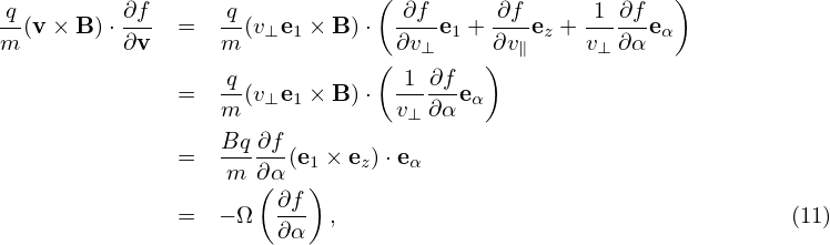
(12)

i.e.,

∂f- -∂f -∂f -∂f ∂f- ∂t +v∥∂z ′ + v⊥cosα∂x ′ + v⊥sinα∂y ′ − Ω∂α = 0.

(13)

Deﬁne the following coordinates transform (guiding-center transform):

( || X = x′ + v⊥-siΩnα, |||| Y = y′ − v⊥cΩosα, ||{ Z = z′, α′ = α, |||| v′∥ = v∥, |||| v′⊥ = v⊥, ( t′ = t

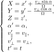(14)

Next, we express the partial derivatives of f appearing in Eq. (13) in terms of the guiding-center coordinates. Using the chain rule, we obtain

∂f- ∂f- ∂X- ∂f-∂Y- ∂f-∂Z- ∂f-∂α-′ ∂f-∂v′∥ -∂f-∂v′⊥- ∂f-∂t′ ∂α = ∂X ∂α + ∂Y ∂ α + ∂Z ∂α + ∂α′ ∂α + ∂v′∥ ∂α + ∂v′⊥ ∂α + ∂t′∂α ∂f ∂X ∂f ∂Y ∂f = --- ---+ ------ + --′ ∂X ∂α ∂Y ∂ α ∂α = ∂f′ v⊥-cosα + ∂f′ v⊥sinα-+ ∂f′. (15) ∂x Ω ∂y Ω ∂α

Similarly, for other derivatives, we obtain

∂f ∂f ---= --′, ∂t ∂t

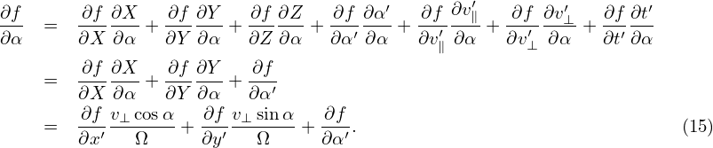
(16)

and

∂f ∂f ∂X ∂f ∂Y ∂f ∂Z ∂f ∂α ′ ∂f ∂v ′ ∂f ∂v′ ∂f ∂t′ --′ = ------′ +-----′ + -----′ +--′---′ +--′--∥′ +--′---⊥′-+ --′--′ ∂z ∂X ∂z ∂Y ∂z ∂Z ∂z ∂α ∂z ∂v∥ ∂z ∂v⊥ ∂z ∂t ∂z ≈ ∂f- × 0+ ∂f-× 0 + ∂f-, (17) ∂X ∂Y ∂Z

where we have assumed that the dependence of X and Y on z′ (via Ω) is weak enough to be neglected. And also

′ ∂v′ ′ ′ ∂f- = ∂f-∂X- + ∂f-∂Y-+ ∂f-∂Z-+ ∂f-∂-α + ∂f- --∥+ -∂f-∂v⊥-+ ∂f-∂t- ∂x′ ∂X ∂x ′ ∂Y ∂x′ ∂Z ∂x′ ∂α′ ∂x′ ∂v′∥ ∂x′ ∂v′⊥ ∂x ′ ∂t′∂x′ ∂f-∂X- ∂f-∂Y- = ∂X ∂x ′ + ∂Y ∂x′ ∂f ∂f ≈ ∂X- ×1 + ∂Y-× 0, (18)

∂f ∂f ---′ ≈--- ∂y ∂Y

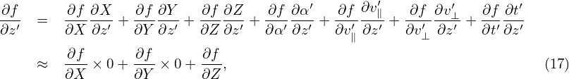
(19)

Using the above results, equation (13) in the guiding-center coordinates is written as

∂f ′∂f ′ ′ ∂f ′ ′ ∂f ( ∂f v⊥ cosα ∂f v⊥ sinα ∂f) ∂t′ + v∥∂Z-+ v⊥cosα ∂X + v⊥ sin α ∂Y-− Ω ∂X- --Ω----+ ∂Y----Ω---+ ∂α-′ = 0.

(20)

Here we ﬁnd some terms cancel each other, giving

∂f ′∂f ( ∂f ) ∂t′ + v∥∂Z-− Ω ∂α′ = 0.

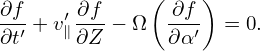(21)

Equation (21) is the equation for f in the guiding-center coordinates (X,Y,Z,v_⊥′,α′,v_∥′).

1.2.1 Gyro-averaging

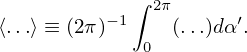
Deﬁne gyro-phase averaging operator

−1∫ 2π ′ ⟨...⟩ ≡ (2π) 0 (...)dα .

(22)

Then averaging Eq. (21) over α′, we get

∂⟨f⟩ ′∂⟨f⟩ −1 ∫ 2π ( ∂f ) ′ -∂t′-+ v∥-∂Z- − (2π) Ω ∂α′ dα = 0. 0

(23)

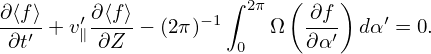
As is assumed above, Ω is approximately independent of α′ and thus Ω in Eq. (23) can be moved outside of the gyro-angle integration, giving

( ) ∂⟨f⟩ ′∂-⟨f⟩ −1∫ 2π ∂f- ′ ∂t′ +v∥ ∂Z − Ω(2π) 0 ∂α′ dα = 0.

(24)

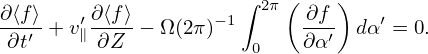
Peforming the integration, we get

∂⟨f⟩ ′∂⟨f⟩ − 1 ′ ′ ∂t′ + v∥ ∂Z − Ω (2π ) [f(α = 2π)− f(α = 0)] = 0.

(25)

Since α′ = 2π and α′ = 0 correspond to the same phase space location, the corresponding values of the distribution function must be equal. Then the above equation reduces to

∂⟨f-⟩ ′∂⟨f⟩ ∂t′ + v∥∂Z = 0,

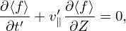(26)

which is an equation for the gyro-angle independent part of the distribution function.

Next let us investigate whether the guiding-center transform can be made use of to simplify the kinetic equation for more general cases where we have a (weakly) non-uniform static magnetic ﬁeld, plus electromagnetic perturbations of low frequency (and of small amplitude and k_∥ρ_i ≪ 1). And we will include the eﬀect that B₀ depends on α′, i.e., grad-B and curvature drift.

[next] [front] [up]