Note that the coefficient before ∂F0∕∂𝜀 in Eq. (133) involves the time derivative of ⟨δϕ⟩α, which is problematic if treated by using explicit finite difference in particle simulations (I test the algorithm that treats this term by implicit scheme, the result roughly agrees with the standard method discussed in Sec. 5.6). It turns out that ∂⟨δΦ⟩α∕∂t can be eliminated by defining another gyro-phase independent function δf by
|
| (135) |
Then, in terms of δf, the perturbed distribution function δF is written as
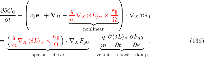 | (136) |
Using Eq. (135) and Eq. (133), the equation for δf is written as
![[ ∂ ]
∂t + (v∥e∥ + VD + δVD )⋅∇X δf
[ ]
− q-∂F0- ∂-+ (v∥e∥ + VD + δVD )⋅∇X ⟨δϕ⟩α
m ∂ 𝜀 ∂[t ]
− q-⟨δϕ⟩ ∂-+ (v e + V + δV )⋅∇ ∂F0-
m α ∂t ∥ ∥ D D X ∂ 𝜀
q ∂⟨δL ⟩α ∂F0
= − δVD ⋅∇XF0 − m- --∂t---∂𝜀- (137)](nonlinear_gyrokinetic_equation145x.png)
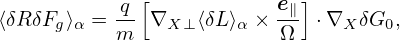
The blue term in expression (136) gives “the polarization density” when integrated in the velocity space (discussed in Sec. 5.6). The reason for the name “polarization” is that (δΦ −⟨δΦ⟩α) is the difference between the local value and the averaged value on a gyro-ring, expressing a kind of “separation”.
![[ ]
-∂ + (ve + V + δV )⋅∇ δf
∂t ∥ ∥ D D X
= − δVD ⋅∇XF0
q [ ∂⟨v⋅δA ⟩α ] ∂F0
− m- − ---∂t----− (v∥e∥ + VD + δVD )⋅∇X ⟨δΦ⟩α ∂𝜀-, (138)](nonlinear_gyrokinetic_equation146x.png)