|
| (215) |
where the parallel currents are given by
 | (216) |
 | (217) |
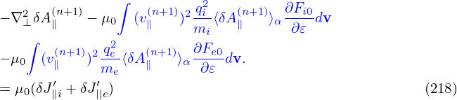
where δJ∥i′ and δJ∥e′ is the parallel current carried by the distribution function δh in Eq. (203), which are updated from the value at the nth time step to the (n + 1)th time step using an explicit scheme and therefore does not depends on the field at the (n + 1)th step. The blue terms in Eqs. (216) and (217) are sometimes called “skin current”, which depend on the unknown field at the (n + 1)th step and thus need to be moved to the left-hand side of Ampere’s law (215) if we want to solve this equation by direct methods. In this case, equation (215) is written as
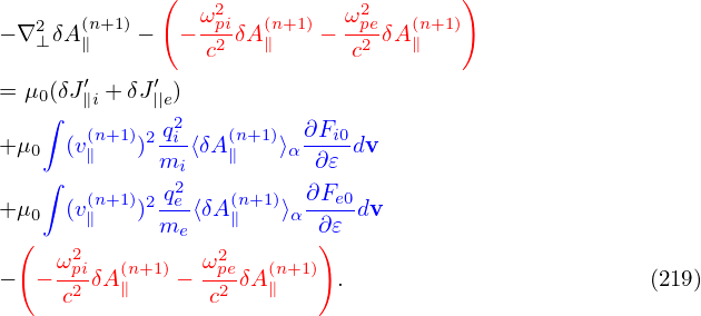
Therefore we go back to Eq. (215) and try to solve it using iterative methods. However, it is found numerically that directly using Eq. (215) as an iterative scheme is usually divergent. To obtain a convergent iterative scheme, we need to have an approximate form for the blue terms, which is independent of markers and so that it is easy to construct its matrix, and then subtract this approximate form from both sides. After doing this, the iterative scheme has better chance to be convergent (partially due to that the right-hand side becomes smaller). An approximate form is that derived by neglecting the FLR effect given in Sec. 4.6. Using this, the iterative scheme for solving Eq. (215) is written as
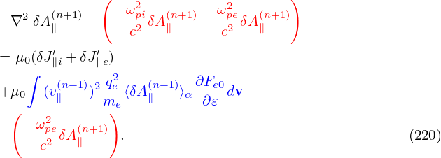
In the drift-kinetic limit (i.e., neglecting the FLR effect), the blue and red terms on the right-hand side of the above equation cancel each other exactly. Even in this case, it is found numerically that these terms need to be retained and the blue terms are evaluated using markers. Otherwise, numerical inaccuracy can give numerical instabilities, which is the so-called cancellation problem. The explanation for this is as follows. The blue terms are part of the current. The remained part of the current carried by δh is computed by using Monte-Carlo integration over markers. If the blue terms are evaluated analytically, rather than using Monte-Carlo integration over markers, then the cancellation between this analytical part and Monte-Carlo part can have large error (assume that there are two large contribution that have opposite signs in the two parts) because the two parts are evaluated using different methods and thus have different accuracy, which makes the cancellation less accurate.Because the ion skin current is less than its electron counterpart by a factor of me∕mi, its accuracy is not important. The cancellation error is not a problem and hence can be neglected. In this case, equation (219) is simplified as
Note that the blue term will be evaluated using Monte-Carlo markers.