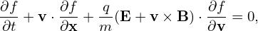
Vlasov equation and dimensionality reduction

1.2 Vlasov equation and dimensionality reduction

The Vlasov equation in terms of particle coordinates (x,v) is written

∂f-+ v ⋅ ∂f-+ q-(E+ v × B) ⋅ ∂f-= 0, ∂t ∂x m ∂v

(1)

where f = f(x,v) is the particle distribution function, x and v are the location and velocity of particles. The distribution function f depends on 7 variables (t,x,v).

Consider a simple case where the electromagnetic ﬁeld is a time-independent and spatial uniform magnetic ﬁeld, B = B₀ and E = 0. Let us examine the Vlasov equation in this simple case and look if there is any coordinate system that can reduce the dimensionality of the problem.

Choose Cartesian coordinate system (x,y,z) for the conﬁguration space. Describe the velocity space using a right-handed cylindrical coordinates (v_⊥,α,v_∥), where v_∥ = v ⋅ e_∥, e_∥ is the unit vector along the magnetic ﬁeld, α is the azimuthal angle of the velocity relative to e_x. Then the 6D phase-space are described by coordinates (x,y,z,v_⊥,α,v_∥). The distribution function f depends on 7 variables, namely x,y,z,v_∥,α,v_⊥, and t.

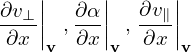
In (x,v_⊥,α,v_∥) coordinates, the gradient in velocity space, ∂f∕∂v, is written as

∂f-= ∂f-e1 + ∂f-ez +-1-∂feα, ∂v ∂v⊥ ∂v∥ v⊥ ∂α

(2)

where e₁ = v_⊥∕|v_⊥| = (v − (v ⋅ e_z)e_z)∕|v − (v ⋅ e_z)e_z| and e_α = −e₁ × e_z. Then -q
m (v × B) ⋅ ∂f
∂v is written as

( ) q- ∂f- q- -∂f- -∂f 1--∂f- m(v × B)⋅ ∂v = m (v⊥e1 × B )⋅ ∂v⊥ e1 + ∂v∥ez + v⊥ ∂αeα ( ) = q-(v⊥e1 × B )⋅-1-∂f-eα m v⊥ ∂α = B0q-∂f(e1 × ez)⋅eα m (∂α ) = − Ω ∂f- , (3) ∂α

where Ω = B₀q∕m is the gyro-frequency. Then the Vlasov equation (1) is written as

∂f ∂f ∂f ∂f ( ∂f) ∂t-+v⊥ cosα∂x-+ v⊥ sinα ∂y-+ v∥ ∂z − Ω ∂α- = 0,

(4)

Deﬁne the following coordinates transform (guiding-center transform):

( (| x′ = x+ v⊥sinα, || x = x ′− v′⊥-sinα′, |||| y′ = y− v⊥Ωcosα, |||| y = y′ + v′⊥-Ωcosα′, |{ z′ = zΩ, |{ z = z′,Ω | α ′ = α, ⇒ | α = α′, |||| v′= v∥, |||| v = v′, |( v∥′= v . ||( ∥ ∥ ⊥ ⊥ v⊥ = v⊥′.

(5)

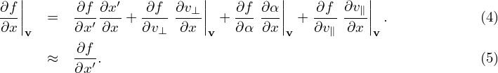
Then, in terms of the new coordinates (x′,y′,z′,v_∥′,v_⊥′,α′), ∂f∕∂α′ is written as

∂f || ∂f ∂x ∂f ∂y ∂f ∂ α --′|| = -----′ +-----′ +------′ ∂α x′,y′,z′,v′∥,v′⊥ ∂x∂α ∂y ∂α ∂ α∂α ∂f-1- ′ ′ ∂f-1- ′ ′ ∂f- = − ∂x Ω v⊥cosα − ∂y Ω v⊥sinα + ∂α ∂f 1 ∂f 1 ∂f = − ∂x-Ω-v⊥cosα − ∂y-Ωv⊥ sinα + ∂α-, (6)

Using this, Eq. (4) is written as

∂f ∂f ( ∂f) ---+ v∥′--′ − Ω ---′ = 0. ∂t ∂z ∂α

(7)

(Note that the derivative ∂f∕∂α′ in the new coordinate system incorporate three derivatives in the original coordinate system, namely, ∂f∕∂x, ∂f∕∂y, and ∂f∕∂α.) Note that x′, y′ and v_⊥′ do not appear in Eq. (7), which means that the grids correspond to these variables are not needed when numerically solving Eq. (7) using Euler grid-based methods, i.e., the dimesion of the problem is reduced. This reduction will reduce the computational cost.

The dimension reduction for the above simple case is found by using the guiding-center transform. This motivates us to investigate whether the guiding-center transform can be made use of to simplify the kinetic equation for more general cases where we have a (weakly) non-uniform static magnetic ﬁeld plus electromagnetic perturbations of low frequency (and of small amplitude and k_∥ρ_i ≪ 1).

[prev] [prev-tail] [front] [up]