In a magnetic field, given a particle location and velocity (x,v), we know how to calculate its guiding-center location X, i.e.,
|
| (8) |
where e∥ = B0∕B0, Ω = qB0∕m, B0 = B0(x) is the equilibrium (macroscopic) magnetic field at the particle position. We will consider Eq. (8) as a transform and call it guiding-center transform[1]. Note that the transform (8) involves both position and velocity of particles.
For later use, define ρ ≡−v × e∥∕Ω, which is the vector gyro-radius pointing from the the guiding-center to the particle position.
Given (x,v), it is straightforward to obtain X by using Eq. (8). On the other hand, the inverse transform, i.e., given (X,v), to find x, which is in principle not easy because Ω and e∥ depend on x, which usually requires solving for the root of a nonlinear equation. Numerically, one can use
 | (9) |
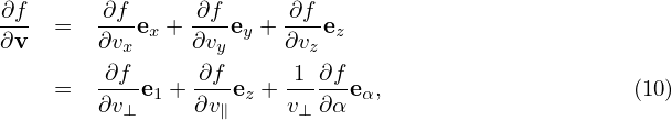
as an iteration scheme to compute x, with the initial guess chosen as x0 = X. The equilibrium magnetic field we will consider has spatial scale length much larger than the thermal gyro radius ρ. In this case the difference between the values of e∥(x)∕Ω(x) and e∥(X)∕Ω(X) is small and thus can be neglected. Then the inverse guiding-center transform can be written as
 | (10) |
which can also be considered as using the iterative scheme (9) to computer x with initial guess of x being X and stopping at the first iteration. [The difference between equilibrium field values evaluated at X and x is always neglected in gyrokinetic theory. Therefore it does not matter whether the above e∥∕Ω is evaluated at x or X. What matters is where the perturbed fields are evaluated: at x or at X. The values of perturbed fields at x or at X are different and this is called the finite Larmor radius (FLR) effect, which is almost all that the gyrokinetic theory is about.]
The inverse guiding-center transformation (10) needs to be performed numerically in gyrokinetic PIC simulations when we deposit markers to grids or when we calculate the gyro-averaged field to be used in pushing guiding-centers.