
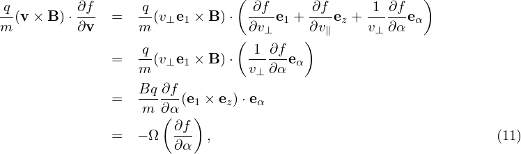
The guiding-center transformations (8) and (10) involve the particle velocity v. It is the cross product between v and e∥(x) or e∥(X) that is actually used. Therefore, only the perpendicular velocity (which is defined by v⊥ = v − v ⋅ e∥) enters the transform. A natural choice of coordinates for the perpendicular velocity is (v⊥,α), where v⊥ = |v⊥| and α is the azimuthal angle of the perpendicular velocity in the local perpendicular plane.
The parallel direction is fully determined by B0(x), but there are degrees of freedom in choosing one of the two perpendicular basis vectors. In order to make the azimuthal angle α fully defined, we need to choose a way to define one of the two perpendicular directions. In GEM simulations, one of the perpendicular direction is chosen as the direction perpendicular to the magnetic surface, which is fully determined at each spatial point. (We need to define the perpendicular direction at each spatial location to make ∂α∕∂x|v defined, which is needed in the Vlasov differential operators. However, it seems that terms related to ∂α∕∂x|v are finally dropped due to that they are of higher order**check.)
In the following, α will be called the “gyro-angle” . [Note that, in the guiding-center coordinates (X,v∥,v⊥,α), α is a velocity coordinate rather than a spatial coordinate. When transformed back to particle coordinates, α is both a velocity coordinate and a spatial coordinate. Consider a series of points in terms of guiding-center coordinates (X,v∥,v⊥,α) with (X,v∥,v⊥) fixed but with α changing. Using the inverse guiding-center transform (10), we know that the above points form a gyro-ring in space, i.e., α influences both particle velocity and location.]
The gyro-angle is an important variable we will stick to because we need to directly perform averaging over this variable (with X fixed) in deriving the gyrokinetic equation. We have more than one choice for the remaining velocity coordinates , such as (v,v∥), or (v,v⊥), or (v∥,v⊥). In Frieman-Chen’s paper, the velocity coordinates other than α are chosen to be (𝜀,μ) defined by
|
| (11) |
and
 | (12) |
where Φ0(x) is the equilibrium (macroscopic) electrical potential.
Note that (𝜀,μ,α) is not sufficient in uniquely determining a velocity vector. An additional parameter σ = sign(v∥) is needed to determine the sign of v∥ = v ⋅e∥. In the following, the dependence of the distribution function on σ is often not explicitly shown in the variable list (i.e., σ is hidden/suppressed), which, however, does not mean that the distribution function is independent of σ.
Another frequently used velocity coordinates are (μ,v∥,α). In the following, I will derive the gyrokinetic equation in (𝜀,μ,α) coordinates. After that, I transform it to (μ,v∥,α) coordinates.
One important thing to note about the above velocity coordinates is that they are defined relative to the local magnetic field. If the field itself is spatially varying (such as in tokamaks), the above velocity coordinates are also spatially varying for a fixed velocity v. Specifically, the following derivatives are nonzero:
 | (13) |