5.14 Verification of the code by using analytic results of Landau damping

One advantage of δf simulation is that nonlinear effects can be readily turned off by setting the particle orbits to the unperturbed orbits (orbits in the equilibrium field), so that the simulation results can be compared with analytic results obtained in the linear case. Choose Maxwellian distribution as the equilibrium velocity distribution function:

(124)

In order to impose a single-k (spatial wavenumber) density perturbation, we set the initial value of δF as

(125)

This perturbation will excite an electrostatic wave and this wave will be damped by a collisionless damping mechanism called Landau damping. Fig. 4 compares the analytic results of Landau damping with those of the linear δf simulation, which shows good agreement between each other in both the frequency and the damping rate.

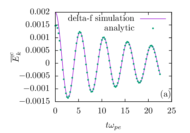
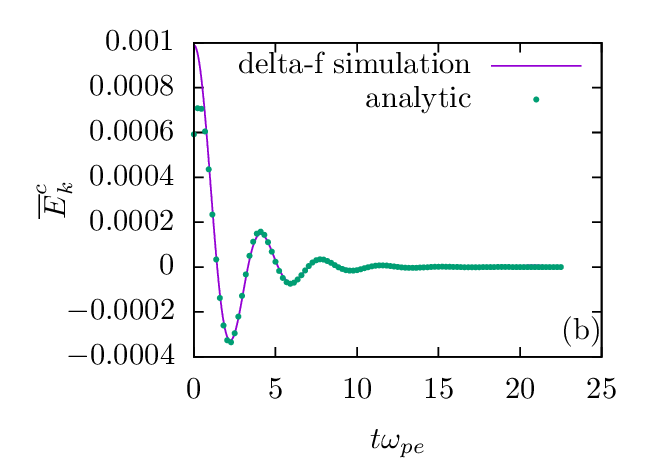
Figure 4: Time evolution of the Fourier cosine component of the electrical field E_k^(c) for (a) k = 8 × 2π∕L  and (b) k = 16 × 2π∕L. Initial value of the δf is set as δf = 0.001sin(kx)exp(−v²∕v_t²)∕. Parameters used in the δf simulations are dt = 0.0125, L∕λ_D = 100, dx∕λ_D = 0.25, and N = 2 × 10⁵. Uniform random sampling of the phase space is used. The difference between the linear and nonlinear δf simulations is negligible and only linear δf simulation results are plotted here. The analytic frequency and damping rate are obtained by numerically solving the electron plasma wave dispersion relation, which is given by 1 + 2²[1 + ζZ(ζ)] = 0,where ζ = ω∕kv_t, v_t = , and Z(ζ) = ∫ _Cdz is the plasma dispersion function[5].

The initial perturbation δF given by Eq. (125) are carried equally by the right-going and left-going particles. As a result of this, the electron plasma wave excited in the simulation is always a standing-wave (a standing wave is composed of two waves with the same frequency and wave-number but opposite propagation directions). Figure 5 plots the spatial structure of the electrical field E_x at four successive time, which clearly shows that the wave excited is a standing wave.

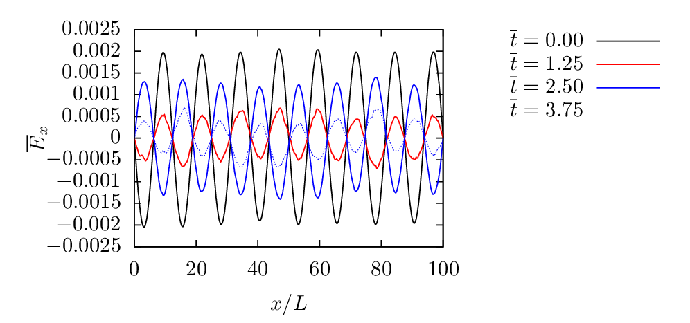
Figure 5: Spatial structure of the electric field at four successive time in the δf simulation with the initial perturbation given by δf = 0.001cos(kx)exp(−v²∕v_t²)∕ with k = 8 × 2π∕L. Other parameters are dt = 0.0125, L∕λ_D = 100, and dx∕λ_D = 0.25; N = 2 × 10⁵ markers with Maxwellian distribution in velocity and uniform distribution in space are loaded.

To excite a right-going wave, instead of a standing-wave, we can set the initial value of δF as

(126)

This initial perturbation is not symmetric about v_x and thus will carry electric current. Unless otherwise specified, the remainder of this note will consider only the symmetrical perturbation of the form (125).