5.15 Methods of identifying resonant particles
Analytically, resonant particles are defined as those particles whose velocity is close to the phase-velocity of the wave.
These particles are expected to exchange more energy with the waves compared with the non-resonant particles. Next, we
examine the phase-space structure of δF in order to find a general way of identifying the resonant region in the
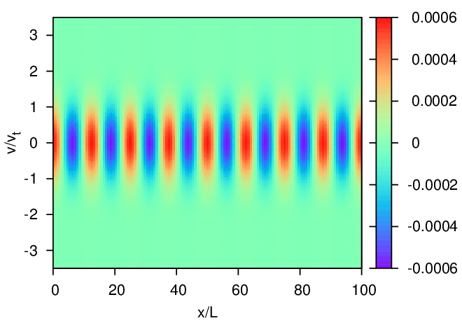
phase-space. The initial phase-space structure of δF is plotted in Fig. 6a, which shows the fluctuation in x direction and
Maxwellian distribution in vx direction. Figure 6b plots the phase-space structure of δF at t = 20∕ωpe. It is not obvious
what kind of useful information can be obtained from the figure. Note that lower velocity particles carry more
perturbation than higher velocity particles because of the exp(−v2∕vt2) dependence in δF. The dominant
structure of δF in the lower velocity region may blur the change of δF in the higher velocity region. To make
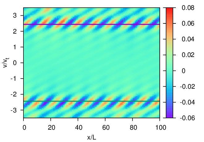
the change of δF obvious, define a new function S(v,x) ≡ δF∕![[exp(− v2∕v2t)∕√π-]](particle_simulation144x.png) , which eliminate the
initial variation of δF in vx direction. Figure 7 plots the contour of S(v,x) in phase space (x,v) at t = 0 and
t = 20∕ωpe, which shows that there are peaks developing near v ≈±2.44 at t = 20∕ωpe. The location of
the peaks of S in the phase-space, v ≈±2.44, is very near the phase-velocity of the wave excited in the
simulation (vp∕vt = ω∕kvt = ±2.44). Therefore, the peaks of S prove to be a good indication of the resonant
region.
, which eliminate the
initial variation of δF in vx direction. Figure 7 plots the contour of S(v,x) in phase space (x,v) at t = 0 and
t = 20∕ωpe, which shows that there are peaks developing near v ≈±2.44 at t = 20∕ωpe. The location of
the peaks of S in the phase-space, v ≈±2.44, is very near the phase-velocity of the wave excited in the
simulation (vp∕vt = ω∕kvt = ±2.44). Therefore, the peaks of S prove to be a good indication of the resonant
region.
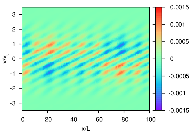
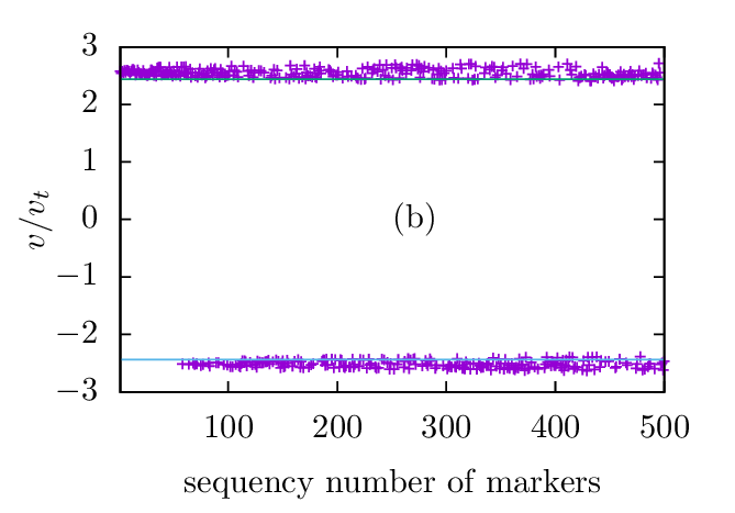
We select the top 500 markers that have large variation in δf∕![[ √ -]
exp(− v2∕v2t)∕ π](particle_simulation148x.png) and then compare their
velocity with the phase-velocity of the wave. The results are plotted in Fig. 8, which confirms that these
velocities are close to the phase-velocity of the wave. Note that, since the wave excited in the simulation is a
standing-wave, which has two opposite phase-velocities, the corresponding resonant velocity also have two opposite
values.
and then compare their
velocity with the phase-velocity of the wave. The results are plotted in Fig. 8, which confirms that these
velocities are close to the phase-velocity of the wave. Note that, since the wave excited in the simulation is a
standing-wave, which has two opposite phase-velocities, the corresponding resonant velocity also have two opposite
values.
There is difference between Fig. 8a and Fig. 8b, which arises from the different sampling of the velocity space. In Fig.
8b, we note that the top 50 resonant particles all have positive velocity, which is nonphysical because there is no preferred
direction in the system with a standing wave and symmetric velocity distribution.
 with
with 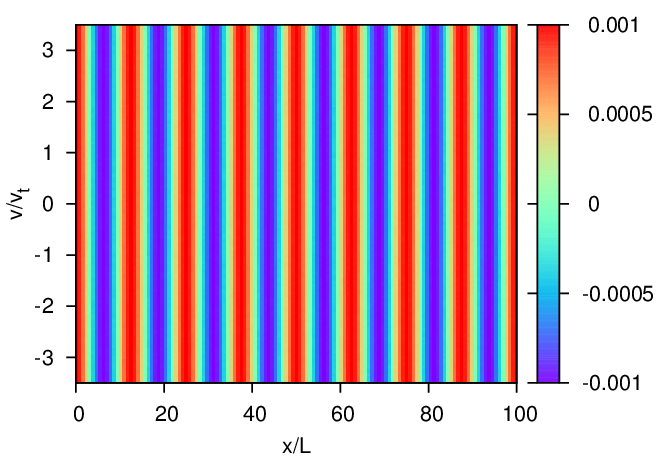
![[ √ -]
exp(− v2∕v2t)∕ π](particle_simulation146x.png) at
at  with
with 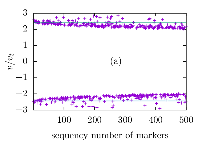
![[ √-]
exp(− v2∕v2t)∕ π](particle_simulation149x.png) between
between  with
with ![[ √ -]
exp(− v2∕v2t)∕ π](particle_simulation151x.png) . The first marker has the largest variation. The solid
lines on the figure indicate the phase-velocity of the wave excited in the simulation (
. The first marker has the largest variation. The solid
lines on the figure indicate the phase-velocity of the wave excited in the simulation (