2.2 Weights of markers

Denote the physical particle distribution function in question by f (f can be the full-f or δf, depending on the context). The weight of a marker in this note is defined as the number of physical particles carried by f in the corresponding phase-space volume sampled by the marker, i.e.,

(14)

which, by using Eq. (5),  is further written as

(15)

or, by using Eq. (11), is written as

(16)

2.2.1 Some discussions

In most PIC codes I wrote, I implement several kinds of marker distribution functions, which can be chosen via an option. In practice, I primarily use the marker distribution g that is uniform in real space and Maxwellian in velocity space with a constant temperature (the other forms of marker distributions are used occasionally for benchmarking purpose), i.e., g is given by

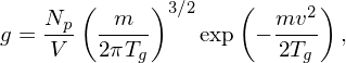(17)

where T_g is a constant temperature, N_p is the number of markers, and V is the spatial volume of the computational box. This marker distribution satisfies the normalization ∫ gdvdr = N_p.

[In the literature on δf PIC simulations, the weight defined by different authors may differ by a factor and this factor is taken into account when calculating velocity moments using the weight. For example, in Ben’s thesis[?], the weight is defined as w_j⋆ = δf∕f₀, where f₀ is the equilibrium physical distribution function. Assume that f₀ is an Maxwellian distribution with constant temperature T_g, then the marker distribution given in Eq. (17) can be written in terms of f₀ as g = N_pf₀∕(n₀V ), where n₀ is the equilibrium number density. Then w_j⋆ and the weight w_j defined above is related by

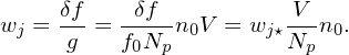(18)

As another example, in the GEM code, the particle weight is defined by w_⋆ = δf∕g_⋆ and g_⋆ is chosen as

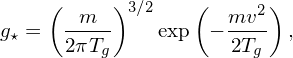(19)

which is related to g defined in Eq. (17) by g = g_⋆N_p∕V . Here g_⋆ satisfies the normalization ∫ g_⋆dvdr = V . Then the relation of w_⋆j in GEM and w_j in this note is given by

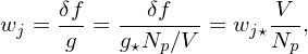(20)

Note that w_j⋆ defined here is of number density dimension. Actually used in the code is the normalized weight defined by w_j⋆ = w_j⋆∕n_u, where n_u is the number density unit used in GEM. Then the relation between w_j and w_j⋆ is given by

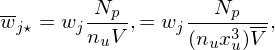(21)

where V = V∕x_u³ and x_u is the length unit used in GEM.]