Metric tensor for general coordinate system

Consider a general coordinate system $(\psi , \theta , \zeta )$. The metric tensor is the transformation matrix between the covariant basis vectors and the contravariant ones. To obtain the metric matrix, we write the contrariant basis vectors in terms of the covariant ones, such as

$$\nabla \psi = a^1 \mathcal{J} \nabla \theta \times \nabla \zeta +... ...a \zeta \times \nabla \psi + a^3 \mathcal{J} \nabla \psi \times \nabla \theta .$$ (140)

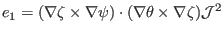
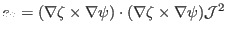
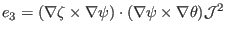
Taking the scalar product respectively with $\nabla \psi$, $\nabla \theta$, and $\nabla \zeta$, Eq. (140) is written as

$$a^1 = \vert \nabla \psi \vert^2,$$ (141)

$$a^2 = \nabla \psi \cdot \nabla \theta,$$ (142)

$$a^3 = \nabla \psi \cdot \nabla \zeta .$$ (143)

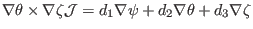
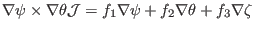
Similarly, we write

$$\nabla \theta = b^1 \mathcal{J} \nabla \theta \times \nabla \zeta... ...la \zeta \times \nabla \psi + b^3 \mathcal{J} \nabla \psi \times \nabla \theta,$$ (144)

Taking the scalar product with $\nabla \psi$, $\nabla \theta$, and $\nabla \zeta$, respectively, the above becomes

$$b^1 = \nabla \theta \cdot \nabla \psi$$ (145)

$$b^2 = \vert \nabla \theta \vert^2,$$ (146)

$$b^3 = \nabla \theta \cdot \nabla \zeta .$$ (147)

The same situation applies for the $\nabla \zeta$ basis vector,

$$\nabla \zeta = c^1 \nabla \theta \times \nabla \zeta \mathcal{J}+... ...imes \nabla \psi \mathcal{J}+ c^3 \nabla \psi \times \nabla \theta \mathcal{J},$$ (148)

Taking the scalar product with $\nabla \psi$, $\nabla \theta$, and $\nabla \zeta$, respectively, the above equation becomes

$$c^1 = \nabla \zeta \cdot \nabla \psi$$ (149)

$$c^2 = \nabla \zeta \cdot \nabla \theta$$ (150)

$$c^3 = \vert \nabla \zeta \vert^2$$ (151)

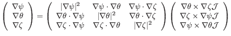
Summarizing the above results in matrix form, we obtain

$$\left(\begin{array}{c} \nabla \psi\\ \nabla \theta\\ \nabla \zeta... ...i \mathcal{J}\\ \nabla \psi \times \nabla \theta \mathcal{J} \end{array}\right)$$ (152)

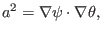
Similarly, to convert contravariant basis vector to covariant one, we write

$$\nabla \theta \times \nabla \zeta \mathcal{J}= d_1 \nabla \psi + d_2 \nabla \theta + d_3 \nabla \zeta$$ (153)

Taking the scalar product respectively with $\nabla \theta \times \nabla \zeta \mathcal{J}$, $\nabla \zeta \times \nabla \psi \mathcal{J}$, and $\nabla \psi \times \nabla \theta \mathcal{J}$, the above equation becomes

$$d_1 = \vert \nabla \theta \times \nabla \zeta \vert^2 \mathcal{J}^2$$ (154)

$$d_2 = (\nabla \theta \times \nabla \zeta \mathcal{J}) \cdot (\nabla \zeta \times \nabla \psi \mathcal{J})$$ (155)

$$d_3 = (\nabla \theta \times \nabla \zeta \mathcal{J}) \cdot (\nabla \psi \times \nabla \theta \mathcal{J})$$ (156)

For the second contravariant basis vector

$$\nabla \phi \times \nabla \psi \mathcal{J}= e_1 \nabla \psi + e_2 \nabla \theta + e_3 \nabla \zeta$$ (157)

$$e_1 = (\nabla \zeta \times \nabla \psi) \cdot (\nabla \theta \times \nabla \zeta) \mathcal{J}^2$$ (158)

$$e_2 = (\nabla \zeta \times \nabla \psi) \cdot (\nabla \zeta \times \nabla \psi) \mathcal{J}^2$$ (159)

$$e_3 = (\nabla \zeta \times \nabla \psi) \cdot (\nabla \psi \times \nabla \theta) \mathcal{J}^2$$ (160)

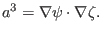
For the third contravariant basis vector

$$\nabla \psi \times \nabla \theta \mathcal{J}= f_1 \nabla \psi + f_2 \nabla \theta + f_3 \nabla \zeta$$ (161)

$$f_1 = (\nabla \psi \times \nabla \theta) \cdot (\nabla \theta \times \nabla \zeta) \mathcal{J}^2$$ (162)

$$f_2 = (\nabla \psi \times \nabla \theta) \cdot (\nabla \zeta \times \nabla \psi) \mathcal{J}^2$$ (163)

$$f_3 = (\nabla \psi \times \nabla \theta) \cdot (\nabla \psi \times \nabla \theta) \mathcal{J}^2$$ (164)

Summarizing these results, we obtain

$$\left(\begin{array}{c} \nabla \theta \times \nabla \zeta \mathcal... ...(\begin{array}{c} \nabla \psi\\ \nabla \theta\\ \nabla \zeta \end{array}\right)$$ (165)

Note that the matrix in Eqs. (152) and (165) should be the inverse of each other. It is ready to prove this by directly calculating the product of the two matrix.