Consider the case that the boundary flux surface is circular with radius  and the center of the cirle at
 . Consider the case
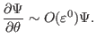
 . Expanding
  in the small parameter
 ,
,
 |
(383) |
where
 ,
,
 .
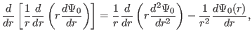
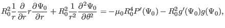
Substituting Eq. (383) into Eq. (382), we obtain
.
Substituting Eq. (383) into Eq. (382), we obtain
Multiplying the above equation by  , we obtain
 |
(384) |
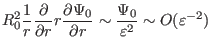
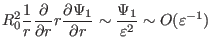
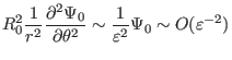
Further assume the following ordering
 |
(385) |
and
 |
(386) |
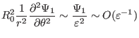
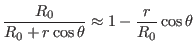
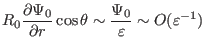
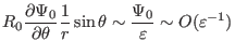
Using these orderings, the order of the terms in Eq. (384) can be
estimated as
 |
(387) |
 |
(388) |
 |
(389) |
 |
(390) |
 |
(391) |
 |
(392) |
 |
(393) |
 |
(394) |
 |
(395) |
The leading order (
 order) balance is given by the
following equation:
order) balance is given by the
following equation:
 |
(396) |
It is reasonable to assume that  is independent of
  since
corresponds to the limit
since
corresponds to the limit
 . (The limit
can have two cases, one is
. (The limit
can have two cases, one is
 , another is
 . In the former case, must be independent of
since should be single-valued. The latter case corresponds to
a cylinder, for which it is reasonable (really?) to assume that is
independent of .) Then Eq. (396) is written
. In the former case, must be independent of
since should be single-valued. The latter case corresponds to
a cylinder, for which it is reasonable (really?) to assume that is
independent of .) Then Eq. (396) is written
 |
(397) |
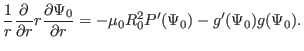
(My remarks: The leading order equation (397) does not correponds
strictly to a cylinder equilibrium because the magnetic field
 depends on .) The
next order (
depends on .) The
next order (
 order) equation is
 |
(398) |
|
(399) |
It is obvious that the simple poloidal dependence of
 will
satisfy the above equation. Therefore, we consider
will
satisfy the above equation. Therefore, we consider  of the form
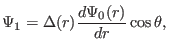 |
(400) |
where
 is a new function to be determined. Substitute this into
the Eq. (), we obtain an equation for
,
is a new function to be determined. Substitute this into
the Eq. (), we obtain an equation for
,
 |
(401) |
 |
(402) |
|
(403) |
|
(404) |
Using the identity
equation () is written as
|
(405) |
Using the leading order equation (), we know that the second and fourth term
on the l.h.s of the above equation cancel each other, giving
 |
(406) |
 |
(407) |
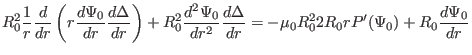
Using the identity
 |
(408) |
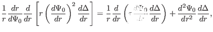
equation (407) is written
![$\displaystyle \frac{1}{r} \frac{d r}{d \Psi_0} \frac{d}{d r} \left[ r \left( \f...
... r} \right] = - \mu_0 2 R_0 r P' (\Psi_0) + \frac{1}{R_0} \frac{d \Psi_0}{d r},$](img1269.png) |
(409) |
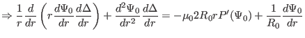
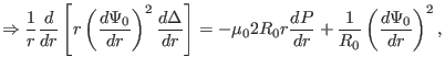 |
(410) |
Using
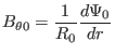 |
(411) |
equation (410) is written
![$\displaystyle \frac{1}{r} \frac{d}{d r} \left[ r B_{\theta 0}^2 \frac{d \Delta}...
...ght] = - \mu_0 2 \frac{1}{R_0} r \frac{d P}{d r} + \frac{B_{\theta 0}^2}{R_0} .$](img1272.png) |
(412) |
 |
(413) |
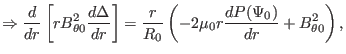
which agrees with equation (3.6.7) in Wessson's book[12].
yj
2018-03-09

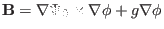
![$\displaystyle R_0^2 \frac{1}{r} \frac{\partial}{\partial r} r \frac{\partial
\...
...0) - \mu_0 R_0^4 P''
(\Psi_0) \Psi_1 - R_0^2 [g' (\Psi_0) g (\Psi_0)]' \Psi_1 $](img1258.png)