Pressure and toroidal field function profile

The function $p (\Psi)$ and $g (\Psi)$ in the GS equation are free functions which must be specified by users before solving the GS equation. Next, we discuss one way to specify the free functions. Following Ref. [9], we take $P (\Psi)$ and $g (\Psi)$ to be of the forms

$$P (\Psi) = P_0 - (P_0 - P_b) \hat{p} (\overline{\Psi}),$$ (441)

$$\frac{1}{2} g^2 (\Psi) = \frac{1}{2} g_0^2 (1 - \gamma \hat{g} (\overline{\Psi})),$$ (442)

with $\hat{p}$ and $\hat{g}$ chosen to be of polynomial form:

$$\hat{p} (\overline{\Psi}) = \overline{\Psi}^{\alpha},$$ (443)

$$\hat{g} (\overline{\Psi}) = \overline{\Psi}^{\beta},$$ (444)

where

$$\overline{\Psi} \equiv \frac{\Psi - \Psi_a}{\Psi_b - \Psi_a},$$ (445)

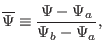
with $\Psi_b$ the value of $\Psi$ on the boundary, $\Psi_a$ the value of $\Psi$ on the magnetic axis, $\alpha$, $\beta$, $\gamma$, $P_0$, $P_b$, and $g_0$ are free parameters. Using the profiles of $P$ and $g$ given by Eqs. (441) and (442), we obtain

$$\frac{d P (\Psi)}{d \Psi} = - \frac{1}{\Delta} (P_0 - P_b) \alpha \overline{\Psi}^{\alpha - 1}$$ (446)

where $\Delta = \Psi_b - \Psi_a$, and

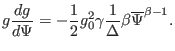$$g \frac{d g}{d \Psi} = - \frac{1}{2} g_0^2 \gamma \frac{1}{\Delta} \beta \overline{\Psi}^{\beta - 1} .$$ (447)

Then the term on the r.h.s (nonlinear source term) of the GS equation is written

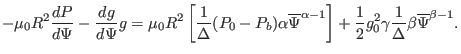$$- \mu_0 R^2 \frac{d P}{d \Psi} - \frac{d g}{d \Psi} g = \mu_0 R^2... ...+ \frac{1}{2} g_0^2 \gamma \frac{1}{\Delta} \beta \overline{\Psi}^{\beta - 1} .$$ (448)

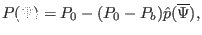
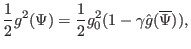
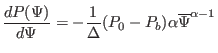
The value of parameters $P_0$, $P_b$, and $g_0$ in Eqs. (441) and (442), and the value of $\alpha$ and $\beta$ in Eqs. (443) and (444) can be chosen arbitrarily. The parameter $\gamma$ is used to set the value of the total toroidal current. The toroidal current density is given by Eq. (62), i.e.,

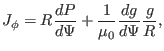$$J_{\phi} = R \frac{d P}{d \Psi} + \frac{1}{\mu_0} \frac{d g}{d \Psi} \frac{g}{R},$$ (449)

which can be integrated over the poloidal cross section within the boundary magnetic surface to give the total toroidal current,

$$I_{\phi} = \int J_{\phi} d S$$

$$= \int \left( R \frac{d P}{d \Psi} + \frac{1}{\mu_0} \frac{d g}{d \Psi} \frac{g}{R} \right) d R d Z$$

$$= \int \left[ R \left( - \frac{1}{\Delta} \right) (P_0 - P_b) \hat{... ...{1}{2} g_0^2 \gamma \frac{1}{\Delta} \hat{g}' (\overline{\Psi}) \right] d R d Z$$ (450)

Using

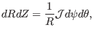$$d R d Z = \frac{1}{R} \mathcal{J}d \psi d \theta,$$ (451)

Eq. (450) is written as

$$I_{\phi} = \int \left[ \left( - \frac{1}{\Delta} \right) (P_0 - P... ...\frac{1}{\Delta} \hat{g}' (\overline{\Psi}) \right] \mathcal{J}d \psi d \theta,$$ (452)

from which we solve for $\gamma$, giving

$$\gamma = \frac{- \Delta I_{\phi} - (P_0 - P_b) \int [\hat{p}' (\o... ... \frac{1}{R^2} \hat{g}' (\overline{\Psi}) \right] \mathcal{J}d \psi d \theta} .$$ (453)

If the total toroidal current $I_{\phi}$ is given, Eq. (453) can be used to determine the value of $\gamma$.