6.4 An example: (ψ,𝜃,ζ) coordinates

Suppose (ψ,𝜃,ζ) is an arbitrary general coordinate system. Following Einstein’s notation, contravariant basis vectors are denoted with upper indices as

(93)

In term of the contravairant basis vectors, A is written

(94)

where the components are easily obtained by taking scalar product with e_ψ,e_𝜃,ande_ζ, yielding A_ψ = A ⋅ e_ψ, A_𝜃 = A ⋅ e_𝜃, and A_ζ = A ⋅ e_ζ. Similarly, in term of the covariant basis vectors, A is written

(95)

where A^ψ = A ⋅ e^ψ, A^𝜃 = A ⋅ e^𝜃, and A^ζ = A ⋅ e^ζ.

Using the above notation, the relation in Eq. (89) is written as

(96)

(97)

(98)

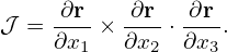
where  𝒥 = [(∇ψ ×∇𝜃) ⋅∇ζ]⁻¹. Similarly, the relation in Eq. (90) is written as

(99)

(100)

(101)