9.1 Finding magnetic surfaces

Two-dimensional data Ψ(R,Z) on a rectangular grids (R,Z) is read from the G_EQDSK file (G-file) of EFIT code. Based on the 2D array data, I use 2D cubic spline interpolation to construct a interpolating function Ψ = Ψ(R,Z). To construct a magnetic surface coordinate system, I need to find the contours of Ψ, i.e., magnetic surfaces. The values of Ψ on the magnetic axis, Ψ₀, and the value of Ψ on the last closed flux surface (LCFS), Ψ_b, are given in G-file. Using these two values, I construct a 1D array “psival” with value of elements changing uniform from Ψ₀ to Ψ_b. Then I try to find the contours of Ψ with contour level value ranging from Ψ₀ to Ψ_b. This is done in the following way: construct a series of straight line (in the poloidal plane) that starts from the location of the magnetic axis and ends at one of the points on the LCFS. Combine the straight line equation, Z = Z(R), with the interpolating function Ψ(R,Z), we obtain a one variable function h = Ψ(R,Z(R)). Then finding the location where Ψ is equal to a specified value Ψ_i, is reduced to finding the root of the equation Ψ(R,Z(R)) − Ψ_i = 0. Since this is a one variable equation, the root can be easily found by using simple root finding scheme, such as bisection method (bisection method is used in GTAW code). 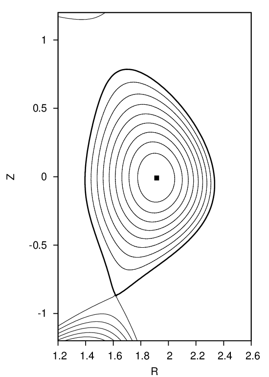After finding the roots for each value in the array “psival” on each straight lines, the process of finding the contours of Ψ is finished. The contours of Ψ found this way are plotted in Fig. 7.

In the above, we mentioned that the point of magnetic axis and points on the LCFS are needed to construct the straight lines. In G-file, points on LCFS are given explicitly in an array. The location of magnetic axis is also explicitly given in G-file. It is obvious that some of the straight lines Z = Z(R) that pass through the location of magnetic axis and points on the LCFS will have very large or even infinite slope. On these lines, finding the accurate root of the equation Ψ(R,Z(R)) −Ψ_i = 0 is difficult or even impossible. The way to avoid this situation is obvious: switch to use function R = R(Z) instead of Z = Z(R) when the slope of Z = Z(R) is large (the switch condition I used is |dZ∕dR| > 1).

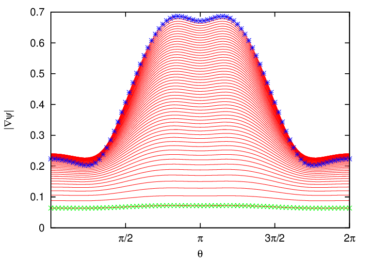
In constructing the flux surface coordinate with desired Jacobian, we will need the absolute value of the gradient of Ψ, |∇Ψ|, on some specified spatial points. To achieve this, we need to construct a interpolating function for |∇Ψ|. The |∇Ψ| can be written as

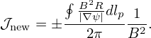(200)

By using the center difference scheme to evaluate the partial derivatives with respect to R and Z in the above equation (using one side difference scheme for the points on the rectangular boundary), we can obtain an 2D array for the value of |∇Ψ| on the rectangular (R,Z) grids. Using this 2D array, we can construct an interpolating function for ∇Ψ by using the cubic spline interpolation scheme.