Expression of metric elements of magnetic coordinates (ψ,𝜃,ϕ)

9.2 Expression of metric elements of magnetic coordinates (ψ,𝜃,ϕ)

Metric elements of the (ψ,𝜃,ϕ) coordinates, e.g., ∇ψ ⋅∇𝜃, are often needed in practical calculations. Next, we express these metric elements in terms of the cylindrical coordinates (R,Z) and their partial derivatives with respect to ψ and 𝜃. Note that, in this case, the coordinate system is (ψ,𝜃,ϕ) while R and Z are functions of ψ and 𝜃, i.e.,

R = R (ψ,𝜃),

(201)

Z = R (ψ,𝜃).

(202)

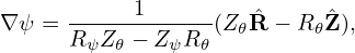
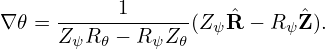
Then ∇R and ∇Z are written as

ˆ ∇R = R = Rψ∇ ψ + R𝜃∇ 𝜃,

(203)

∇Z = ˆZ = Zψ∇ ψ + Z𝜃∇𝜃,

(204)

wehre R_ψ ≡ ∂R∕∂ψ, etc. Equations (203) and (204) can be solved to give

1 ∇ψ = R-Z--−-Z-R--(Z 𝜃Rˆ − R 𝜃ˆZ), ψ 𝜃 ψ 𝜃

(205)

-----1------ ˆ ˆ ∇𝜃 = ZψR 𝜃 − R ψZ𝜃(ZψR − R ψZ).

(206)

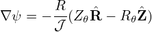
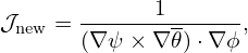
Using the above expressions, the Jacobian of (ψ,𝜃,ϕ) coordinates, 𝒥 , is written as

−1 𝒥 = ∇ψ × ∇𝜃 ⋅∇ϕ = −-------1-------(Z R ˆϕ − R Z ˆϕ)× ϕˆ (RψZ 𝜃 − ZψR 𝜃)2 𝜃 ψ 𝜃 ψ R 1 = −(Z𝜃R-ψ −-R-𝜃Z-ψ)R, (207)

i.e.,

𝒥 = R (R 𝜃Zψ − R ψZ𝜃).

(208)

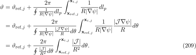
Using this, Expressions (205) and (206) are written as

R ∇ ψ = − 𝒥 (Z 𝜃Rˆ− R 𝜃ˆZ)

(209)

and

∇𝜃 = R-(ZψRˆ− R ψˆZ). 𝒥

(210)

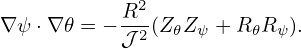
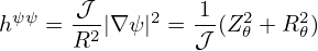
Then the elements of the metric matrix are written as

R2 |∇ψ|2 = 𝒥2(Z2𝜃 + R2𝜃),

(211)

|∇ 𝜃|2 = R2-(Z2 +R2 ), 𝒥 2 ψ ψ

(212)

and

2 ∇ψ ⋅∇ 𝜃 = − R-(Z 𝜃Z ψ + R 𝜃Rψ). 𝒥2

(213)

Equations (211), (212), and (213) are the expressions of the metric elements in terms of R, R_ψ, R_𝜃, Z_ψ, and Z_𝜃. [Combining the above results, we obtain