Contravariant form of magnetic ﬁeld in (ψ,𝜃,ζ) coordinates

Recall that the contravariant form of the magnetic ﬁeld in (ψ,𝜃,ϕ) coordinates is given by Eq. (157), i.e.,

B = − Ψ′(∇ϕ × ∇ψ + ˆq∇ψ × ∇ 𝜃).

(260)

Next, let us derive the corresponding form in (ψ,𝜃,ζ) coordinates. Using the deﬁnition of ζ, equation (260) is written as

B = − Ψ ′∇ (ζ + qδ)× ∇ψ − Ψ′ˆq∇ψ × ∇ 𝜃 ′ ′ ′ = − Ψ ∇ ζ × ∇ ψ − Ψ ∇ (qδ) × ∇ψ − Ψ ˆq∇ψ × ∇𝜃 = − Ψ ′∇ ζ × ∇ ψ − Ψ ′q∂-δ∇𝜃 × ∇ψ − Ψ′ˆq∇ψ × ∇𝜃 (261) ∂ 𝜃

Using Eq. (253), the above equation is simpliﬁed as

B = − Ψ′(∇ζ × ∇ψ + q∇ψ × ∇ 𝜃). (262)

Equation (262) is the contravariant form of the magnetic ﬁeld in (ψ,𝜃,ζ) coordinates.

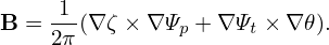
The expression of the magnetic ﬁeld in Eq. (262) can be rewritten in terms of the ﬂux function Ψ_p and Ψ_t discussed in Sec. 11.2. Equation (262) is

B = ∇ Ψ × ∇ ζ + q∇ 𝜃× ∇ Ψ,

(263)

which, by using Eq. (237), i.e., ∇Ψ = ∇Ψ_p∕(2π), is rewritten as

1 B = 2π-(∇ζ ×∇ Ψp + q∇ Ψp × ∇ 𝜃),

(264)

which, by using Eq. (244), i.e., q = dΨ_t∕dΨ_p, is further written as

1 B = --(∇ ζ × ∇ Ψp + ∇ Ψt × ∇𝜃). 2π

(265)