13.7 Numerical verification of the field-aligned coordinates
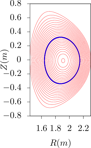
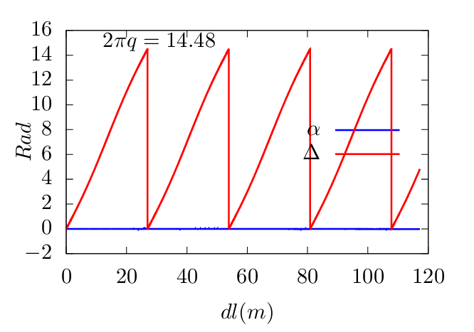
The generalized toroidal angle α is numerically calculated in my code. To verify B ⋅∇α = 0 along a
magnetic field-line, figure 26 plots the values of α along a magnetic field line, which indicates that α is
constant. This indicates the numerical implementation of the field-aligned coordinates is
correct.
Binormal wavenumber
Let us introduce the binormal wavenumber, which is frequently used in presenting turbulence
simulation results. Define the binormal direction s by
s =  , ,
|
which is a unit vector lying on a magnetic surface and perpendicular to B. The binormal wavenumber
of a mode is defined by
 | (339) |
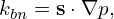
where p is the phase of the mode. Consider a mode given by exp(ikψψ + im𝜃 − inζ), then the phase
p = kψψ + m𝜃 − nζ. Then kbn is written as
where the radial phase kψψ does not appear since B ×∇Ψ ⋅∇ψ = 0. The above expression can be
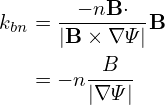
further written as Equation (341) is the general expression of the binormal wavenumber. On the resonant surface of the
mode, i.e., q(ψ) = m∕n, then the above expression is written as
![nB ⋅
kbn = |B-×∇-Ψ|[q∇Ψ × ∇𝜃 − ∇Ψ × ∇ ζ].](tokamak_equilibrium438x.png) | (342) |
Using Eq. (262), i.e., B = −(∇ζ ×∇Ψ + q∇Ψ ×∇𝜃), the above expression is written as
Using Bp = |∇Ψ|∕R, the above equation is written
 | (343) |
which indicates the binormal wavenumber generally depends on the poloidal angle. For large
aspect-ratio tokamak, we have Bϕ ≈ B, q ≈ Bϕr∕(BpR). Then Eq. (343) is written
 | (344) |
which indicates the binormal wavenumber are approximately independent of the poloidal angle. Since
m = nq on a resonant surface, the above equation is written |kbn|≈ m∕r, which is the usual poloidal
wave number. Due to this relation, the binormal wavenumber kbn is often called the poloidal
wavenumber and denoted by k𝜃 in papers on tokamak turbulence. In the GENE code, y coordinate is
defined by y = αr0∕q0. Then the ky of a mode of toroidal mode number n is given by ky = 2π∕λy
where λy = λαr0∕q0 and λα = 2π∕n. Then ky is written as ky = nq0∕r0, which is similar
to the binormal defined above. For this reason, ky of GENE code is also called binormal
wave-vector, which is in fact not reasonable because neither ∂r∕∂y or ∇y is along the binormal
direction.
 d𝜃.
d𝜃.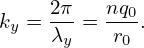
![kbn =----1--- [mB × ∇Ψ ⋅∇ 𝜃− nB × ∇Ψ ⋅∇ ζ]
|B × ∇Ψ |
----1---
= |B × ∇Ψ |[mB ⋅∇Ψ × ∇ 𝜃− nB ⋅∇Ψ × ∇ ζ]
nB⋅ [m ]
= |B-×-∇Ψ-| n-∇Ψ × ∇ 𝜃− ∇ Ψ × ∇ ζ . (341)](tokamak_equilibrium437x.png)