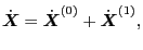
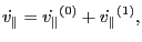
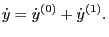
Next, we derive the linearized version of Eq. (77). The
perturbation in electromagnetic field causes perturbation in both distribution
function and particle orbits
 ,
,
 , and
, and
 . Thus we write
 |
(81) |
 |
(82) |
 |
(83) |
 |
(84) |
and substitute this into Eq. (77), we obtain
 |
(85) |
The zero order equation is
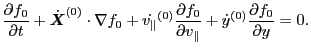 |
(86) |
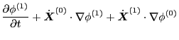
The first order equation is
![$\displaystyle \frac{\partial f_1}{\partial t} + \dot{\ensuremath{\boldsymbol{X}...
...\partial v_{\parallel}} + \dot{y}^{(1)} \frac{\partial f_0}{\partial y} \right]$](img176.png) |
(87) |
Define
 |
(88) |
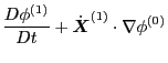
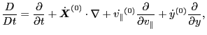
which is the unperturbed orbit propagator, then Eq. (87) is
written as
![$\displaystyle \frac{D f_1}{D t} = - \left[ \dot{\ensuremath{\boldsymbol{X}}}^{(...
...partial v_{\parallel}} + \dot{y}^{(1)} \frac{\partial f_0}{\partial y} \right],$](img178.png) |
(89) |
which agrees with Eq. (21) in Porcelli's paper[1].
At this point, I would like to discuss the equilibrium distribution function.
We know that functions of constants of the motion are solutions to the kinetic
equation. Noting that
 ,
,
 , and
, and  are
constants of the motion in equilibrium field. Then
are
constants of the motion in equilibrium field. Then
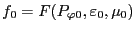 is a solution to the kinetic equation Eq.
(77). Noting that the right-hand side of Eq. (89)
contains partial derivative with respect to variables
is a solution to the kinetic equation Eq.
(77). Noting that the right-hand side of Eq. (89)
contains partial derivative with respect to variables
 , we would like to transform the partial derivatives with
respect to
to one with respect to
, we would like to transform the partial derivatives with
respect to
to one with respect to
 . The right-hand side of Eq.
(89) can be written term by term as
. The right-hand side of Eq.
(89) can be written term by term as
Using these results, Eq. (89) is written as
which can be arranged in the form
![$\displaystyle \frac{D f_1}{D t} = - \left[ \left( \dot{\ensuremath{\boldsymbol{...
...{X}}}^{(1)} \cdot \nabla B_0 \right) \frac{\partial F}{\partial \mu_0} \right],$](img194.png) |
(93) |
which agrees with Eq. (22) in Porcelli's paper[1]. Next, we
need to express
 ,
,
 , and
, and
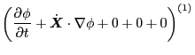
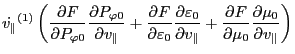
 in terms of the perturbed electromagnetic field. Let us first
consider the coefficient befor the
in terms of the perturbed electromagnetic field. Let us first
consider the coefficient befor the
 term
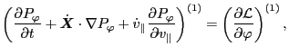
in Eq. (93). We note that Eq. (35) takes the following
form:
term
in Eq. (93). We note that Eq. (35) takes the following
form:
 |
(94) |
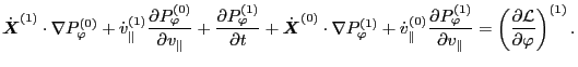
whose linearized version is (noting that
 ,
,
 , and
, and  is time independent, thus
 ,
,
 ,
and
,
and
 are all zeros)
 |
(95) |
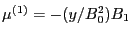
where
 . Using
(Note that
 here denotes total time derivative along the
unperturbed orbit, instead of the perturbed orbit ) in Eq. (95) gives
here denotes total time derivative along the
unperturbed orbit, instead of the perturbed orbit ) in Eq. (95) gives
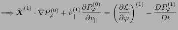
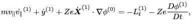 |
(97) |
where, for notation ease, we have defined
 |
(98) |
Equation (97) agrees with Eq. (30) in Porcelli's
paper[1]. The right-hand side of Eq. (97)
provides the desired expression for the coefficent before the
term of Eq. (93).
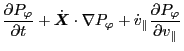
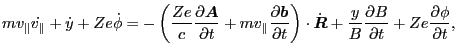
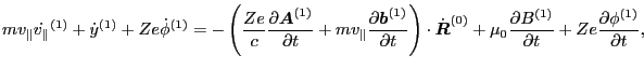
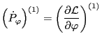
The first order equation of Eq. (52) is written as (Noting that we
are considering toroidal symmetrical equilibrium, thus terms such as
 ,
,
 , and
, and
 are all zeros.)
 |
(99) |
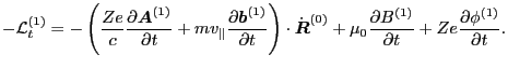
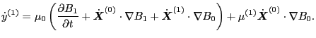
Using this in the Euler equation (43), we obtain
 |
(100) |
Note that
 |
(101) |
then
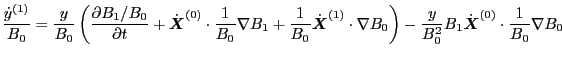
Using this in Eq. (100), we obtain
 |
(102) |
which can be further written as
 |
(103) |
 |
(104) |
The right-hand side of Eq. (104) gives desired expression for the
coefficient before the term
 of Eq.
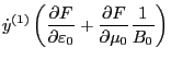
(93). The linearized version of Eq. (32)
of Eq.
(93). The linearized version of Eq. (32)
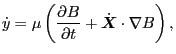 |
(105) |
is written as
 |
(106) |
Noting that
,
 , the above
equation is written as
, the above
equation is written as
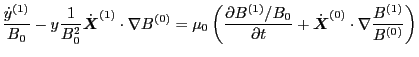
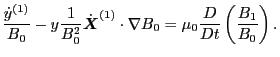
 |
(107) |
 |
(108) |
![$\displaystyle \frac{\dot{y}^{(1)}}{B_0} - y \frac{1}{B_0^2} \dot{\ensuremath{\b...
...} \nabla B^{(1)} - B^{(1)} \cdot \frac{1}{B_0^2} \nabla B^{(0)} \right) \right]$](img234.png) |
(109) |
 |
(110) |
 |
(111) |
Eq. (111) agrees with Eq. (31) in Porceli's paper. The right-hand
side of Eq. (111) provide the desired expression for the coefficient
before
 term in Eq. (93). Using Eqs.
(97), (104), and (111), Eq. (93) is
finally written as
term in Eq. (93). Using Eqs.
(97), (104), and (111), Eq. (93) is
finally written as
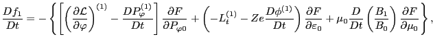 |
(112) |
YouJun Hu
2014-05-19


![$\displaystyle \frac{D f_1}{D t} = - \left[ \dot{\ensuremath{\boldsymbol{X}}}^{(...
...epsilon_0} + \frac{\partial F}{\partial
\mu_0} \frac{1}{B_0} \right) \right], $](img193.png)