Perturbed Lagrangian for ideal MHD perturbation

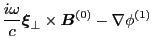
For ideal MHD perturbation, the perturbed magnetic field is written as

$$\ensuremath{\boldsymbol{B}}^{(1)} = \nabla \times \left( \ensuremath{\boldsymbol{\xi}}_{\perp} \times \ensuremath{\boldsymbol{B}}_0 \right)$$ (142)

$$= - \ensuremath{\boldsymbol{B}}_0 \left( \nabla \cdot \ensuremath{\... ...nsuremath{\boldsymbol{\xi}}_{\perp} \cdot \nabla \ensuremath{\boldsymbol{B}}_0,$$ (143)

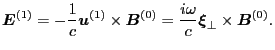
Using Eq. (142), the vector potential of magnetic perturbation is written as

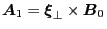$$\ensuremath{\boldsymbol{A}}_1 = \ensuremath{\boldsymbol{\xi}}_{\perp} \times \ensuremath{\boldsymbol{B}}_0$$ (144)

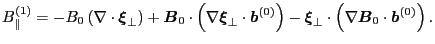
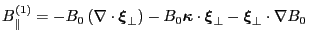
Using Eq. (143), the parallel component of the magnetic perturbation is written as

$$B_{\parallel}^{(1)} \equiv \ensuremath{\boldsymbol{b}}^{(0)} \cdot \ensuremath{\boldsymbol{B}}^{(1)}$$

$$= - B_0 \left( \nabla \cdot \ensuremath{\boldsymbol{\xi}}_{\perp} \... ...a \ensuremath{\boldsymbol{B}}_0 \right] \cdot \ensuremath{\boldsymbol{b}}^{(0)}$$ (145)

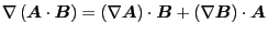
Here I have some important remarks about tensor identities (I had not known these identities before CaiHuiShan told me). First we note the associate law applies in this case (Important!), thus

$$B_{\parallel}^{(1)} = - B_0 \left( \nabla \cdot \ensuremath{\bold... ...\ensuremath{\boldsymbol{B}}_0 \cdot \ensuremath{\boldsymbol{b}}^{(0)} \right) .$$ (146)

Second we have the tensor identity (Important!, CaiHuiShan let me know this identity),

$$\nabla \left( \ensuremath{\boldsymbol{A}} \cdot \ensuremath{\bold... ...t( \nabla \ensuremath{\boldsymbol{B}} \right) \cdot \ensuremath{\boldsymbol{A}}$$ (147)

Using this, the second term of Eq. (146) is written as

$$\ensuremath{\boldsymbol{B}}_0 \cdot \left( \nabla \ensuremath{\boldsymbol{\xi}}_{\perp} \cdot \ensuremath{\boldsymbol{b}} \right) = \ensuremath{\boldsymbol{B}}_0 \cdot \left[ \nabla \left( \ensurem... ...\ensuremath{\boldsymbol{b}} \cdot \ensuremath{\boldsymbol{\xi}}_{\perp} \right]$$

$$= \ensuremath{\boldsymbol{B}}_0 \cdot \left[ 0 - \nabla \ensuremath{\boldsymbol{b}} \cdot \ensuremath{\boldsymbol{\xi}}_{\perp} \right]$$

$$= - B_0 \ensuremath{\boldsymbol{\kappa}} \cdot \ensuremath{\boldsymbol{\xi}}_{\perp},$$ (148)

where $\ensuremath{\boldsymbol{\kappa}} = \ensuremath{\boldsymbol{b}} \cdot \nabla \ensuremath{\boldsymbol{b}}$. The last term of Eq. (146) is written as

$$\ensuremath{\boldsymbol{\xi}}_{\perp} \cdot \left( \nabla \ensuremath{\boldsymbol{B}}_0 \cdot \ensuremath{\boldsymbol{b}} \right) = \ensuremath{\boldsymbol{\xi}}_{\perp} \cdot \left[ \nabla (B_0 \ensuremath{\boldsymbol{b}}) \cdot \ensuremath{\boldsymbol{b}} \right]$$

$$= \ensuremath{\boldsymbol{\xi}}_{\perp} \cdot \left[ ( \ensuremath{... ...\nabla \ensuremath{\boldsymbol{b}}) \cdot \ensuremath{\boldsymbol{b}} \right] .$$ (149)

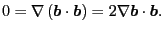
We note that $\nabla \ensuremath{\boldsymbol{b}} \cdot \ensuremath{\boldsymbol{b}} = 0$ (CaiHuiShan let me know this), since the tensor identity in Eq. (147) indicates

$$0 = \nabla \left( \ensuremath{\boldsymbol{b}} \cdot \ensuremath{\... ...ght) = 2 \nabla \ensuremath{\boldsymbol{b}} \cdot \ensuremath{\boldsymbol{b}} .$$ (150)

(It is interesting to note that $\ensuremath{\boldsymbol{b}} \cdot \nabla \ensuremath{\boldsymbol{b}} \equiv \ensuremath{\boldsymbol{\kappa}} \neq 0$ while the above result proves that $\nabla \ensuremath{\boldsymbol{b}} \cdot \ensuremath{\boldsymbol{b}} = 0$.) Thus Eq. (149) becomes

$$\ensuremath{\boldsymbol{\xi}}_{\perp} \cdot \left( \nabla \ensuremath{\boldsymbol{B}}_0 \cdot \ensuremath{\boldsymbol{b}} \right) = \left. \ensuremath{\boldsymbol{\xi}}_{\perp} \cdot \left[ ( \ensu... ...th{\boldsymbol{b}} \nabla B_0 \right) \cdot \ensuremath{\boldsymbol{b}} \right]$$

$$= \ensuremath{\boldsymbol{\xi}}_{\perp} \cdot \nabla B_0$$ (151)

Using the above results, the parallel component of the perturbed magnetic field Eq. (146) becomes

$$B_{\parallel}^{(1)} = - B_0 \left( \nabla \cdot \ensuremath{\bold... ...ldsymbol{\xi}}_{\perp} - \ensuremath{\boldsymbol{\xi}}_{\perp} \cdot \nabla B_0$$ (152)

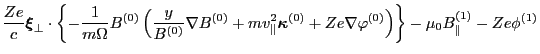
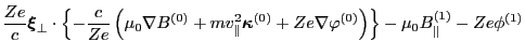
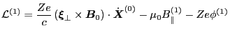
The perturbed Lagrangian, Eq. (133), is

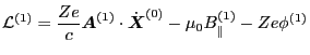$$\mathcal{L}^{(1)} = \frac{Z e}{c} \ensuremath{\boldsymbol{A}}^{(1... ...\ensuremath{\boldsymbol{X}}}^{(0)} - \mu_0 B_{\parallel}^{(1)} - Z e \phi^{(1)}$$ (153)

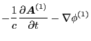
Using Eq. (144) in Eq. (153) yields

$$\mathcal{L}^{(1)} = \frac{Z e}{c} \left( \ensuremath{\boldsymbol{... ...\ensuremath{\boldsymbol{X}}}^{(0)} - \mu_0 B_{\parallel}^{(1)} - Z e \phi^{(1)}$$ (154)

Using Eq. (78) for $\dot{\ensuremath{\boldsymbol{X}}}^{(0)}$, Eq. (154) is written as

$$\mathcal{L}^{(1)} = \frac{Z e}{c} \left( \ensuremath{\boldsymbol{\xi}}_{\perp} \times... ...ldsymbol{E}}^{(0)} \right) \right] - \mu_0 B_{\parallel}^{(1)} - Z e \phi^{(1)}$$

$$= \frac{Z e}{c} \left( \ensuremath{\boldsymbol{\xi}}_{\perp} \times... ...abla \varphi^{(0)} \right) \right] - \mu_0 B_{\parallel}^{(1)} - Z e \phi^{(1)}$$

$$= \frac{Z e}{c} \ensuremath{\boldsymbol{\xi}}_{\perp} \cdot \left\{... ...phi^{(0)} \right) \right] \right\} - \mu_0 B_{\parallel}^{(1)} - Z e \phi^{(1)}$$

$$= \frac{Z e}{c} \ensuremath{\boldsymbol{\xi}}_{\perp} \cdot \left\{... ...} \left( \ldots . \right) \right\} - \mu_0 B_{\parallel}^{(1)} - Z e \phi^{(1)}$$

$$= \frac{Z e}{c} \ensuremath{\boldsymbol{\xi}}_{\perp} \cdot \left\{... ...bla \varphi^{(0)} \right) \right\} - \mu_0 B_{\parallel}^{(1)} - Z e \phi^{(1)}$$

$$= \frac{Z e}{c} \ensuremath{\boldsymbol{\xi}}_{\perp} \cdot \left\{... ...bla \varphi^{(0)} \right) \right\} - \mu_0 B_{\parallel}^{(1)} - Z e \phi^{(1)}$$

$$= - \ensuremath{\boldsymbol{\xi}}_{\perp} \cdot \left( \mu_0 \nabla... ...+ Z e \nabla \varphi^{(0)} \right) - \mu_0 B_{\parallel}^{(1)} - Z e \phi^{(1)}$$

$$= - m v_{\parallel}^2 \ensuremath{\boldsymbol{\xi}}_{\perp} \cdot \... ...^{(1)} + \ensuremath{\boldsymbol{\xi}}_{\perp} \cdot \nabla \phi^{(0)} \right),$$ (155)

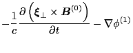
Equation (155) agrees with Eq. (55) in Porcelli's paper[1]. The perturbed electrical field is

$$\ensuremath{\boldsymbol{E}}^{(1)} = - \frac{1}{c} \ensuremath{\bo... ...ensuremath{\boldsymbol{\xi}}_{\perp} \times \ensuremath{\boldsymbol{B}}^{(0)} .$$ (156)

On the other hand, $\ensuremath{\boldsymbol{E}}^{(1)}$ can be expressed as

$$\ensuremath{\boldsymbol{E}}^{(1)} = - \frac{1}{c} \frac{\partial \ensuremath{\boldsymbol{A}}^{(1)}}{\partial t} - \nabla \phi^{(1)}$$

$$= - \frac{1}{c} \frac{\partial \left( \ensuremath{\boldsymbol{\xi}}... ...imes \ensuremath{\boldsymbol{B}}^{(0)} \right)}{\partial t} - \nabla \phi^{(1)}$$

$$= \frac{i \omega}{c} \ensuremath{\boldsymbol{\xi}}_{\perp} \times \ensuremath{\boldsymbol{B}}^{(0)} - \nabla \phi^{(1)}$$ (157)

Comparing Eqs. (156) and (157), we obtain

$$\nabla \phi^{(1)} = 0.$$ (158)

which indicates the perturbed scalar potential is a constant. We can choose $\phi^{(1)} = 0$. We consider the case that there is no electrical field in the equilibrium, i.e., $\phi^{(0)} = 0$. Using $\phi^{(0)} = 0$ and $\phi^{(1)} = 0$, the Lagrangian in Eq. (155) is written as

$$\mathcal{L}^{(1)} = - m v_{\parallel}^2 \ensuremath{\boldsymbol{\... ...allel} + \ensuremath{\boldsymbol{\xi}}_{\perp} \cdot \nabla B_0 \right) \mu_0 .$$ (159)

Substituting the expression of $B_{\parallel}^{(1)}$ in Eq. (152) into the above equation, we obtain

$$\mathcal{L}^{(1)} = - m v_{\parallel}^2 \ensuremath{\boldsymbol{\xi}}_{\perp} \cdot \... ...abla B_0 + \ensuremath{\boldsymbol{\xi}}_{\perp} \cdot \nabla B_0 \right) \mu_0$$

$$= - m v_{\parallel}^2 \ensuremath{\boldsymbol{\xi}}_{\perp} \cdot \... ...{\boldsymbol{\kappa}} \cdot \ensuremath{\boldsymbol{\xi}}_{\perp} \right) \mu_0$$

$$= - \left( m v_{\parallel}^2 - \mu_0 B_0 \right) \ensuremath{\bolds... ...dsymbol{\kappa}} + \mu_0 B_0 \nabla \cdot \ensuremath{\boldsymbol{\xi}}_{\perp}$$ (160)

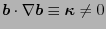
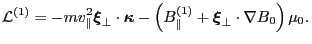
We note an important fact that magnetic curvature $\ensuremath{\boldsymbol{\kappa}}$ is perpendicular to $\ensuremath{\boldsymbol{b}}$. This is because that $\ensuremath{\boldsymbol{\kappa}} \equiv \ensuremath{\boldsymbol{b}} \cdot \nab... ... - \ensuremath{\boldsymbol{b}} \times \nabla \times \ensuremath{\boldsymbol{b}}$. The last equality is due to the vector identity $\nabla \left( \ensuremath{\boldsymbol{A}} \cdot \ensuremath{\boldsymbol{B}} \right)$= $\ensuremath{\boldsymbol{A}} \times \nabla \times \ensuremath{\boldsymbol{B}} +... ...mbol{A}} + \ensuremath{\boldsymbol{B}} \cdot \nabla \ensuremath{\boldsymbol{A}}$. Using this fact, Eq. (160) can also be written as

$$\mathcal{L}^{(1)} = - \left( m v_{\parallel}^2 - \mu_0 B_0 \right... ...ymbol{\kappa}} + \mu_0 B_0 \nabla \cdot \ensuremath{\boldsymbol{\xi}}_{\perp} .$$ (161)

Eq. (161) agrees with Eq. (58) in Porcelli's paper[1].