Evaluate the reconstructed function at discrete points

Evaluate h(t) given by Eq. (42) at the discrete point t = jΔ, yielding

⌊N∑∕2 ( ) N∑−1 ( )⌋ h(jΔ ) = -1 ⌈ Hn exp − in2πj + Hn exp − i(n−-N-)2πj ⌉ . N n=0 N n=N∕2 N ⌊N∕2 ( ) N−1 ( )⌋ -1 ⌈∑ n2πj- ∑ n2πj- ⌉ = N Hn exp − i N + Hn exp − i N . [n=0 n=N∕2 ] -1 N∑−1 ( n2πj-) = N Hn exp − i N + HN ∕2exp(− iπj) . (43) n=0

Drop the blue term (which is negligible if h satisﬁes the condition requried by the sampling theorem), then h(jΔ) is written as

N∑−1 ( ) h (jΔ ) ≈-1 Hn exp − in2πj . N n=0 N

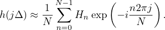(44)

The right-hand side of Eq. (44) turns out to be the inverse DFT discussed in Sec. 4.3.