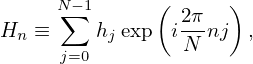
The DFT in Eq. (34), i.e.,
|
| (45) |
with j = 0,1,2,…,N − 1 and n = 0,1,2,…,N − 1 can also be considered as a set of linear algebraic equations for hj and can be solved in terms of hj, which gives
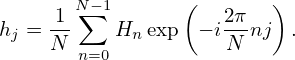 | (46) |
(The details on how to solve Eq. (34) to obtain the solution (46) is provided in Sec. 4.4.) Equation (46) recovers hj from Hn (i.e., the DFT of hj), and thus is called the inverse DFT.
The normalization factor multiplying the DFT and inverse DFT (here 1 and 1∕N) and the signs of the exponents are merely conventions. The only requirement is that the DFT and inverse DFT have opposite-sign exponents and that the product of their normalization factors be 1∕N. In most FFT computer libraries, the 1∕N factor is omitted. So one must take this factor into account when one wants to reproduce the original data after a forward and then a backward transform.