H Drift-kinetic limit

In the drift-kinetic limit, ⟨v⊥⋅δE⟩α = 0, ⟨δB∥v⊥⟩α = 0, and ⟨δh⟩α = δh, where δh is an arbitrary field quantity. Using these, gyrokinetic equation (347) is written as

[ ∂  (                   δB   )    ]
 -- +  v∥e∥ + vD + vE +v∥--⊥- ⋅∇X   δf
 ∂t (           )        B0  [(                 )    ]
= −  vE + v δB⊥-  ⋅∇XF0 − -q   v e + vD + v δB⊥-  ⋅δE ∂F0-.     (392)
           ∥ B0           m     ∥ ∥        ∥ B0        ∂𝜀

H.1 Linear case

Neglecting the nonlinear terms, drift-kinetic equation (392) is written

[ ∂-                 ]
  ∂t + (v∥e∥ + vD) ⋅∇X δf
    (       δB  )          q                ∂F
= −   vE +v∥---⊥  ⋅∇XF0  − --[(v∥e∥ + vD )⋅δE]-0.           (393)
             B0            m                ∂ 𝜀

Next let us derive the parallel momentum equation from the linear drift kinetic equation (this is needed in my simulation). Multiplying the linear drift kinetic equation (393) by qv∥ and then integrating over velocity space, we obtain

∂δj∥     ∫
 ∂t  = − q  dvv∥(v∥e∥ + vD )⋅∇X δf
        ∫     (        δB   )         q  ∫                    ∂F
     − q  dvv∥  vE + v∥ --⊥- ⋅∇XF0  − --q  dvv∥[(v∥e∥ + vD)⋅δE ]--0.  (394)
                       B0            m                        ∂𝜀

Equation (394) involve ∇Xδf and this should be avoided in particle methods whose goal is to avoid directly evaluating the derivatives of δf over phase-space coordinates. On the other hand, the partial derivatives of velocity moment of δf are allowed. Therefore, we would like to make the velocity integration of δf appear. Note that ∇Xδf here is taken by holding (𝜀,μ) constant and thus v∥ is not a constant and thus can not be moved inside ∇X. Next, to facilitate performing the integration over v∥, we transform the linear drift kinetic equation (393) into variable (X,μ,v∥).

H.2 Transform from (X,μ,𝜀) to (X,μ,v∥) coordinates

The kinetic equation given above is written in terms of variable (X,μ,𝜀). Next, we transform it into coordinates (X′,μ′,v∥) which is defined by

 ′
X (X,μ,𝜀) = X,
(395)

μ′(X,μ,𝜀) = μ,
(396)

and

           ∘ -------------
v∥(X, μ,𝜀) =  2(𝜀 − μB0(X )).
(397)

Use this, we have

∂δG0-     ∂X′∂-δG0   ∂μ′∂δG0-  ∂v∥∂-δG0-
∂X  |μ,𝜀 = ∂X  ∂X ′ + ∂X  ∂μ′ + ∂X  ∂v∥
          ∂δG0       ∂ δG0    μ ∂B0 ∂δG0
       =  ∂X-′ |μ,v∥ + 0-∂μ′-− v-dX-∂v--,               (398)
                              ∥      ∥

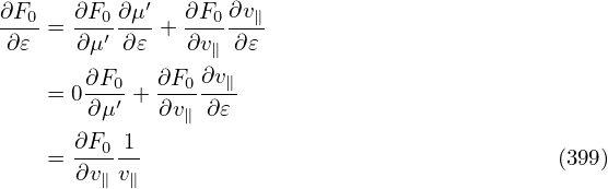
and

∂F    ∂F ∂ μ′  ∂F  ∂v
--0-= --0′--- + --0---∥
∂𝜀    ∂μ  ∂𝜀   ∂v∥ ∂𝜀
    = 0∂F0-+ ∂F0∂v∥
       ∂μ′   ∂v∥ ∂𝜀
      ∂F0-1
    = ∂v∥v∥                                   (399)

Then, in terms of variable (X′,μ,v∥), equation (393) is written

 ∂δf                           ∂ δf
 ∂t-+ (v∥e∥ + vD )⋅∇δf − e∥ ⋅μ∇B-∂v∥
    (           )        (          )              [(        )    ]
= −   vE + v∥δB-⊥ ⋅∇F0 +   vE-+ δB⊥-  ⋅μ∇B ∂F0-− -q   e∥ + vD  ⋅δE  ∂F0,(400)
             B0            v∥    B0        ∂v∥   m         v∥       ∂v∥

where ∇≡ ∂∕∂X′|μ,v∥.

H.3 Parallel momentum equation

Multiplying the linear drift kinetic equation (400) by qv∥ and then integrating over velocity space, we obtain

       ∫                          ∫
∂δj∥+ q   dvv (v e + v  )⋅∇  δf − q  dvv e ⋅μ∇B  ∂δf-
 ∂t          ∥ ∥ ∥   D     X           ∥ ∥      ∂v∥
    ∫      (       δB ⊥)           ∫     ( vE   δB⊥ )      ∂F0
= − q  dvv∥ vE + v∥-B0-  ⋅∇XF0 + q   dvv∥  v--+ -B0-  ⋅μ∇B ∂v--
     ∫     [(        )    ]                 ∥                ∥
−-qq   dvv∥  e∥ + vD- ⋅δE  ∂F0-.                                  (401)
 m                v∥       ∂v ∥

Consider the simple case that F0 does not carry current, i.e., F0(X,μ,v∥) is an even function about v∥. Then it is obvious that the integration of the terms in red in Eq. (401) are all zero. Among the rest terms, only the following term

     ∫
  q-                 ∂F0-1-
− m q  dvv∥[(v∥e∥)⋅δE ]∂v∥v∥
(402)

explicitly depends on δE. Using dv = 2πBdv∥dμ, the integration in the above expression can be analytically performed, giving

    ∫
−-qq   dvv∥[(v∥e∥)⋅δE]∂F0-1
 m                   ∂v∥v∥
   q2 ∫               ∂F0
= −m-   2πBdv∥dμv∥δE ∥∂v∥-
    2 ∫          ∫
= − q   2πBd μδE∥  v∥∂F0-dv∥
   m             (    ∂v∥    )
   q2 ∫               ∫
= −m    2πBd μδE∥  0−   F0dv∥
  q2
= --δE∥n0.                                        (403)
  m

Using these results, the parallel momentum equation (401) is written

                  ∫                         ∫
∂δj∥   q2                                                 ∂δf-
 ∂t  = m δE∥n0 − q  dvv∥(v∥e∥ + vD)⋅∇X δf + q  dvv∥e∥ ⋅μ ∇B ∂v∥
         ∫      (  δB  )         ∫      (δB  )       ∂F
       − q  dvv∥ v∥---⊥  ⋅∇F0 + q   dvv∥ ---⊥  ⋅μ∇B  --0,         (404)
                    B0                    B0         ∂v∥

where the explicit dependence on δE is via the first term q2n0δE∥∕m, with all the the other terms being explicitly independent of δE (δf and δB implicitly depend on δE).

Equation (404) involve derivatives of δf with respect to space and v∥ and these should be avoided in the particle method whose goal is to avoid directly evaluating these derivatives. Using integration by parts, the terms involving ∂∕∂v∥ can be simplified, yielding

                 ∫                                  ∫
∂δj∥= q2δE  n − q  dvv (v e + v  )⋅∇  δf − q(e ⋅∇B )  μδf dv
 ∂t    m   ∥ 0         ∥ ∥ ∥   D    X        ∥    0
         ∫     (   δB⊥-)         ( δB-⊥-)       ∫
      − q  dvv∥  v∥ B0   ⋅∇F0 − q  B0   ⋅(∇B0 )  μF0dv,          (405)

Define p⊥0 = ∫ mv⊥2F0∕2dv and δp⊥ = ∫ mv⊥2δf∕2dv, then the above equation is written

        2         ∫
∂-δj∥ = q-δE ∥n0 − q  dvv∥(v∥e∥ + vD) ⋅∇X δf − q(e∥ ⋅∇B0 ) δp⊥
 ∂t    m  ∫     (       )         (    )             mB0
       − q  dvv   v δB⊥- ⋅∇F  − q  δB-⊥  ⋅(∇B  ) p⊥0-,          (406)
               ∥   ∥B0       0      B0        0 mB0

Next, we try to eliminate the spatial gradient of δf by changing the order of integration. The second term on the right-hand side of Eq. (406) is written
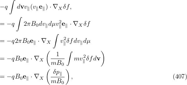
  ∫
− q  dvv ∥(v∥e∥)⋅∇X δf,
    ∫
= − q  2πB  dv dμv2e ⋅∇  δf
          0  ∥   ∥ ∥   X
               ∫  2
= − q2πB0e∥ ⋅∇X  v∥δfdv∥dμ
             (  1  ∫         )
= − qB0e∥ ⋅∇X  ----  mv2∥δfdv
             ( mB0 )
= − qB0e∥ ⋅∇X  δp∥- ,                             (407)
               mB0

where δp∥ = ∫ mv∥2δfdv. Similarly, the term −q ∫ dvv∥(     )
 v∥δBB0⊥-⋅∇XF0 is written as

   ∫     (       )
− q  dvv  v  δB-⊥- ⋅∇  F
        ∥  ∥ B0      X  0
     ∫          (  2δB⊥ )
= − q  2πB0dv∥dμ  v∥-B0-  ⋅∇XF0
     (    )        ∫
= − q δB-⊥  ⋅B0∇X    (v2∥F02πdv∥dμ)
     ( B0 )        [  ∫          ]
= − q δB-⊥  ⋅B ∇    1-  (mv2F dv)
       B0     0  X  B      ∥ 0
             ( p∥0 )
= − qδB ⊥ ⋅∇X mB0-                                  (408)

where p∥0 = ∫ mv∥2F0dv. Similarly, the term −q ∫ dvv∥vD ⋅∇Xδf can be written as the gradient of moments of δf. Let us work on this. The drift vD is given by

      B0vΩ∥∇-×-b-    -μ--
vD =     B ⋆   v∥ + ΩB ⋆B0 × ∇B0.
           ∥           ∥
(409)

where B∥⋆ = B0(             )
 1 + v∥Ωb ⋅∇ × b (refer to my another notes).  Using b ⋅∇× b ≈ 0, we obtain B∥⋆ ≈ B. Then vD is written

      2
vD =  v∥-∇ ×b + μ-b × ∇B0.
      Ω        Ω

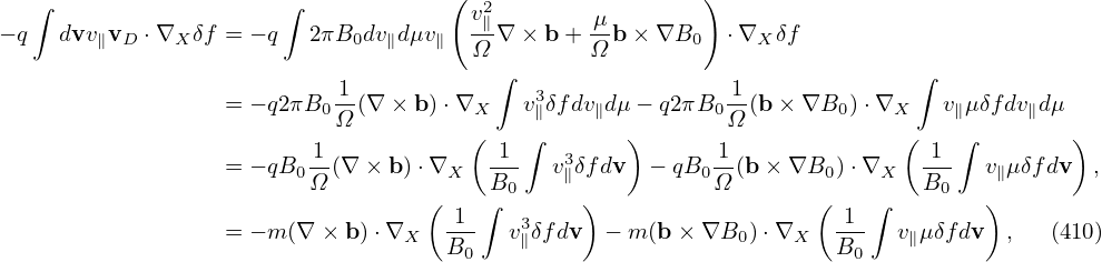
Using this and dv = 2πB0dv∥dμ, the term −q ∫ dvv∥vD ⋅∇Xδf is written as
                                     (                   )
  ∫                    ∫              v2∥        μ
− q  dvv∥vD ⋅∇X δf = − q 2πB0dv ∥dμv∥  -Ω∇ × b + Ω-b ×∇B0   ⋅∇X δf
                                        ∫                                  ∫
                  = − q2πB0-1(∇ × b)⋅∇X    v3∥δf dv∥dμ − q2πB0-1(b ×∇B0 )⋅∇X    v∥μδfdv∥dμ
                           Ω          (    ∫       )       Ω              (   ∫         )
                         1-             -1-   3           -1               -1-
                  = − qB0Ω (∇ × b)⋅∇X   B0   v∥δfdv  − qB0Ω (b× ∇B0 )⋅∇X   B0   v∥μδfdv  ,
                                   ( 1 ∫  3     )                  ( 1 ∫        )
                  = − m(∇ × b)⋅∇X   B--  v∥δfdv  − m (b× ∇B0 )⋅∇X   B--  v∥μδfdv  ,   (410)
                                      0                               0

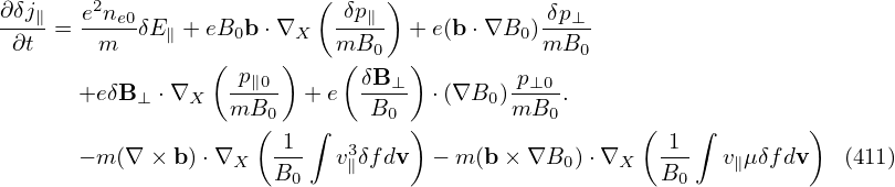
which are the third order moments of δf and may be neglect-able (a guess, not verified). Using the above results, the linear parallel momentum equation is finally written

       2                  (    )
∂δj∥-= e-ne0δE∥ +eB0b ⋅∇X   -δp∥  + e(b⋅∇B0 )-δp⊥
∂t      m        (     )   mB(0   )          mB0
                  -p∥0       δB-⊥         p⊥0-
      +eδB ⊥ ⋅∇X  mB0    +e   B0   ⋅(∇B0 )mB0 .
                     ( 1 ∫       )                  (  1 ∫        )
      − m (∇ × b)⋅∇X  B--  v3∥δfdv  − m (b × ∇B0 )⋅∇X   B--  v∥μδfdv   (411)
                        0                              0

Define

       (     )
        -p∥0    ∇B0- p⊥0-
D0 = ∇  mB0   +  B0  mB0 ,
(412)

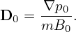
which, for the isotropic case (p∥0 = p⊥0 = p0), is simplified to

     ∇p0-
D0 = mB0 .
(413)

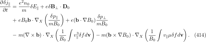
then Eq. (411) is written as

        2
∂δj∥=  en0-δE∥ + eδB ⊥ ⋅D0
 ∂t     m       (    )
    + eB0b ⋅∇X   -δp∥  + e(b⋅∇B0 )-δp⊥
                 mB0(    ∫       ) mB0              (    ∫        )
                     -1-   3                         -1-
    − m (∇ × b)⋅∇X   B0   v∥δfdv  − m (b × ∇B0 )⋅∇X   B0   v∥μδfdv  . (414)

H.4 Special case in uniform magnetic field

In the case of uniform magnetic field, the parallel momentum equation (411) is written as

∂δj∥   q                        δB⊥
-∂t- = m-qE∥ne0 − qe∥ ⋅∇X (δp∥)− q-B-⋅∇Xp ∥0.
                                  0
(415)

H.5 Electron perpendicular flow

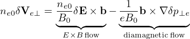
Using the gyrokinetic theory and taking the drift-kinetic limit, the perturbed perpendicular electron flow, δVe⊥, is written (see Sec. F or Appendix in Yang Chen’s paper[1])

n δV    = ne0δE ×b − -1-b × ∇ δp
 e0  e⊥   B◟0-◝◜---◞  e◟B0--◝◜---⊥e◞
           E×B flow     diamagneticflow
(416)

where ne0 is the equilibrium electron number density, δpe⊥ is the perturbed perpendicular pressure of electrons.


Drift kinetic equation

Drift kinetic equation is written

∂f   (           δE × b)       (  e             ) ∂f
-∂t +  v∥b˜+ vD + --B0--  ⋅∇f +  − m-δE∥ − μb˜⋅∇B  ∂v∥ = 0,
(417)

where f = f(x,μ,v∥,t), μ = mv⊥2∕B0 is the magnetic moment, ˜b = b + δB⊥∕B0, b = B0∕B0 is the unit vector along the equilibrium magnetic field, vD = vD(x,μ,v∥) is the guiding-center drift in the equilibrium magnetic field. δE and δB are the perturbed electric field and magnetic field, respectively.

Parallel momentum equation

Multiplying the drift kinetic equation () by v∥ and then integrating over velocity space, we obtain

∫           ∫   (                 )          ∫   (                )
  ∂fev∥dv +   v∥  v∥˜b + vD + δE-×-b  ⋅∇fedv +   v∥ − e-δE∥ − μ ˜b⋅∇B  ∂fedv = 0,
    ∂t                        B0                    m               ∂v∥
(418)

which can be written as

          (                  )
∂J∥e-  ∫       ˜       δE-×-e∥          ∫    (  e-      ˜     ) ∂fe
∂t  +   v∥  v∥b + vD +   B0     ⋅∇fedv +   v∥ − m δE ∥ − μb ⋅∇B  ∂v∥dv = 0,
(419)

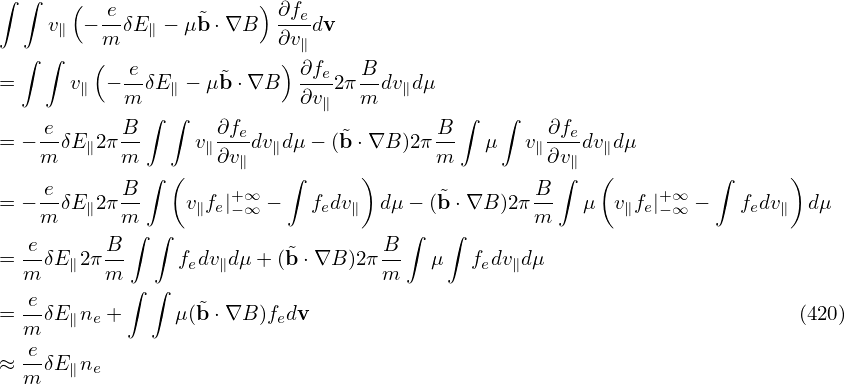
Using dv = B−12πmdv∥dμ, the last term on the RHS of the above equation is written
∫ ∫    (                )
     v∥ − e-δE ∥ − μ˜b ⋅∇B  ∂fedv
          m               ∂v∥
  ∫ ∫    (  e-      ˜     ) ∂fe  B-
=      v∥ − m δE ∥ − μb ⋅∇B  ∂v∥2πm dv∥dμ
    e      B  ∫ ∫   ∂f                  B ∫   ∫   ∂f
= − --δE∥2π--     v∥--edv∥dμ − (˜b ⋅∇B )2π-  μ   v∥--edv∥dμ
    m      m  ∫ (   ∂v∥   ∫      )      m         ∂v∫∥  (         ∫      )
= − e-δE 2πB-    v f |+∞  −   fdv   dμ− (˜b ⋅∇B )2πB-  μ  v f |+∞  −   fdv   dμ
    m   ∥  m      ∥ e−∞       e ∥                m       ∥ e− ∞      e ∥
  -e      B-∫ ∫           ˜        B-∫   ∫
= m δE ∥2πm      fedv∥dμ + (b ⋅∇B )2πm    μ  fedv∥dμ
   e        ∫ ∫
= m-δE ∥ne +    μ(˜b ⋅∇B )fedv                                             (420)
   e
≈ m-δE ∥ne
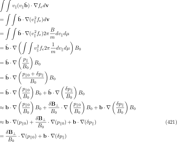
∫ ∫
    v∥(v∥˜b)⋅∇fedv
  ∫ ∫
=     ˜b ⋅∇(v2f )dv
            ∥ e
  ∫ ∫ ˜     2     B-
=     b ⋅∇(v∥fe)2π m dv∥dμ
      ( ∫ ∫       1      )
= ˜b⋅∇       v2∥fe2π--dv∥dμ  B0
      (   )       m
= ˜b⋅∇   p∥- B0
      ( B0      )
  ˜     p∥0 +-δp∥
= b⋅∇      B0     B0
      ( p∥0)          (δp∥)
= ˜b⋅∇   --- B0 + ˜b ⋅∇  ---  B0
      ( B0 )           B0(   )          (   )
≈ b⋅∇   p∥0 B0 + δB-⊥ ⋅∇  p∥0  B0 + b ⋅∇  δp∥- B0
        B0        B0      B0              B0
             δB⊥-
≈ b⋅∇ (p∥0)+  B0  ⋅∇ (p∥0)+ b ⋅∇(δp∥)                        (421)
  δB⊥-
=  B0 ⋅∇ (p∥0)+ b ⋅∇ (δp∥)

where use has been made of b ⋅∇p∥0 = 0.

∂-δJe∥     e-       δB-⊥
  ∂t  = − m δE ∥ne − B0  ⋅∇(p∥0)− b⋅∇ (δp∥)
(422)

Using Eq. () in Eq. (), we obtain

                                [                        ]
   e-                            δB-⊥
μ0em δE∥ne + b ⋅∇ × ∇ × δE = − μ0e B0  ⋅∇(pe∥0) +b ⋅∇ (δpe∥)
(423)


————–


                      (                                      )
                          δB⊥-         -q
− b⋅∇ × ∇ × δE = − μ0e − qB0  ⋅∇Xp ∥0 + m qE∥ne0 − qe∥ ⋅∇X (δp∥) .
(424)


ddddd

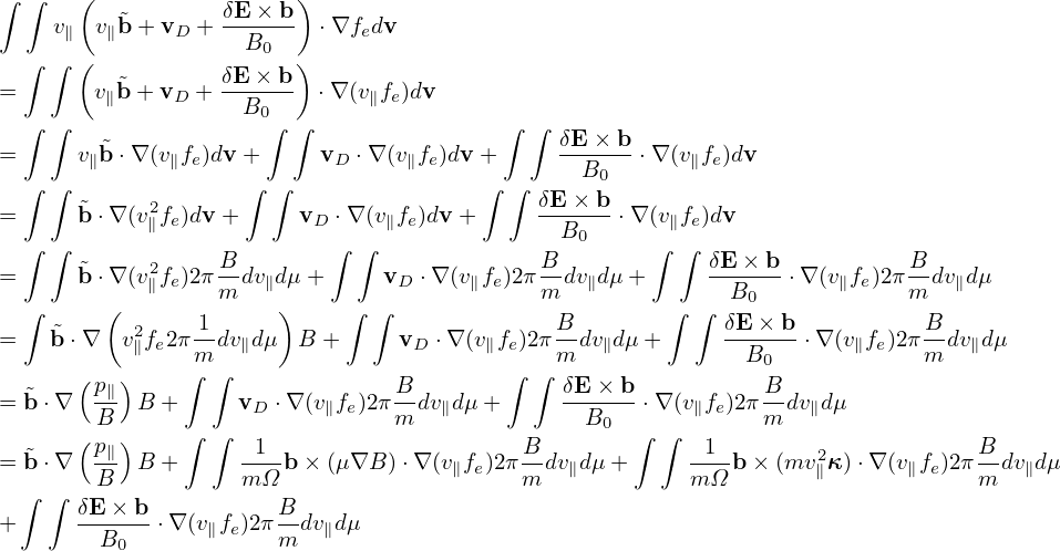
∫ ∫   (                 )
    v   v ˜b+ v  + δE-×-b  ⋅∇f dv
     ∥   ∥    D     B0        e
  ∫ ∫ (   ˜       δE-×-b)
=       v∥b+ vD +   B0    ⋅∇ (v∥fe)dv
  ∫ ∫                 ∫ ∫                ∫  ∫ δE × b
=     v∥˜b ⋅∇(v∥fe)dv +     vD ⋅∇ (v∥fe)dv+      ------ ⋅∇ (v∥fe)dv
  ∫ ∫               ∫ ∫                 ∫ ∫     B0
=     ˜b ⋅∇(v2∥fe)dv+      vD ⋅∇ (v∥fe)dv +    δE-×-b ⋅∇(v∥fe)dv
  ∫ ∫                      ∫ ∫                B0      ∫ ∫
=     ˜b ⋅∇(v2fe)2πB-dv dμ+     vD ⋅∇ (v fe)2πB-dv dμ +     δE-×-b ⋅∇(v fe)2π B-dvdμ
  ∫      (  ∥     m   ∥)    ∫  ∫       ∥    m   ∥      ∫ ∫  B0       ∥     m  ∥
    ˜      2    1-                            B-           δE-×-b           B-
=   b ⋅∇  v∥fe2πm dv∥dμ B +      vD ⋅∇(v∥fe)2π m dv∥dμ +       B0   ⋅∇ (v∥fe)2πm dv∥dμ
      ( p∥)    ∫ ∫              B         ∫ ∫ δE × b           B
= ˜b⋅∇   B- B +      vD ⋅∇ (v∥fe)2πm-dv∥dμ +     --B--- ⋅∇(v∥fe)2π m-dv∥dμ
      ( p )    ∫ ∫                               0  ∫ ∫
= ˜b⋅∇   -∥ B +      -1-b × (μ∇B )⋅∇ (v∥fe)2π B-dv∥dμ+      -1-b × (mv2∥κ)⋅∇ (v∥fe)2πB-dv∥dμ
  ∫ ∫   B           mΩ                     m             mΩ                     m
+     δE-×-b ⋅∇(v∥fe)2π B-dv∥dμ
        B0             m