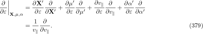
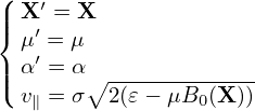
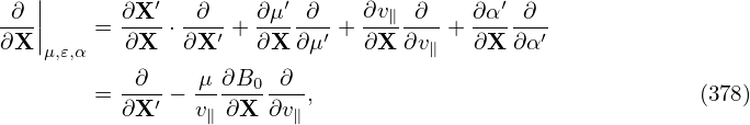
The gyrokinetic equation given above is written in terms of variables (X,μ,𝜀,α). Next, we transform it into coordinates (X′,μ′,v∥,α′) which are defined by
| (377) |
Use this definition and the chain rule, we obtain
and
Then, in terms of (X′,μ′,v∥,α′), equation (135) is written
Dropping terms of order higher than O(λ2), equation (380) is written as
![[ ]
∂- -∂-- ∂B0-∂δG0-
∂t + (v∥e∥ + VD + δVD )⋅∂X ′ δG0 − e∥ ⋅μ∂X ∂v∥
(∂F0 ) ( ∂B0 q ∂⟨δL⟩α) ∂F0 1
= − δVD ⋅ ∂X-′ + δVD ⋅μ ∂X--− m---∂t-- ∂v--v-, (381)
∥ ∥](nonlinear_gyrokinetic_equation440x.png)
The above equation drops all terms higher than O(λ2) and as a result the coefficient before ∂δf∕∂v∥ contains only the mirror force, i.e., −e∥⋅ μ∇B0, which is independent of any perturbations.
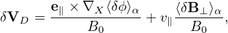
Note that the gyro-averaging operator in (X′,μ′,v∥,α′) coordinates is identical to that in the old coordinates since the perpendicular velocity variable μ is identical between the two coordinate systems. Also note that the perturbed guiding-center velocity δVD is given by
| (382) |
where ∂∕∂X (rather than ∂∕∂X′) is used. Since δϕ(x) = δϕg(X,μ′,α′), which is independent of v∥, then Eq. (378) indicates that ∂δϕ∕∂X = ∂δϕ∕∂X′.
Following the same procedures, equation (143) in terms of (X′,μ′,v∥,α′) is written as
next, try to recover the equation in Mishchenk’s paper:
![[ ∂ ∂ ] ∂δf
-- + (v∥e∥ + VD + δVD )⋅---′ δf − e∥ ⋅μ∇B0----
∂t ( ) ∂X ∂v∥
= − δV ⋅ -∂F0 + δV ⋅μ∇B ∂F0-1-
D ∂X ′ D 0∂v ∥v∥
q [ ∂⟨δA ∥⟩α ( VD ⟨δB ⊥⟩α) ] ∂F0
− m- − --∂t---− e∥ +-v--+ --B---- ⋅∇X ⟨δϕ⟩α ∂v--.
∥ 0 ∥](nonlinear_gyrokinetic_equation443x.png)
δL = δΦ − v ⋅ δA,
| (384) |
![[ ( ) ]
−-q − ∂⟨δA∥⟩α − e∥ + VD-+ -q∇X ⟨A∥⟩α × e∥ ⋅∇X ⟨δϕ⟩α ∂F0.
m ∂t v∥ m Ω ∂v∥](nonlinear_gyrokinetic_equation445x.png)
![[ (h) ( ) ]
− -q − ∂⟨δA∥--⟩α-− VD--+ -q∇ ⟨A ⟩ × e∥ ⋅∇ ⟨δϕ⟩ ∂F0.
m ∂t v∥ m X ∥ α Ω X α ∂v∥](nonlinear_gyrokinetic_equation446x.png)
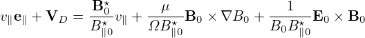
The guiding-center velocity in the equilibrium field is given by
| (385) |
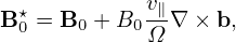
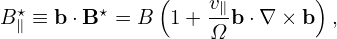
where
| (386) |
| (387) |
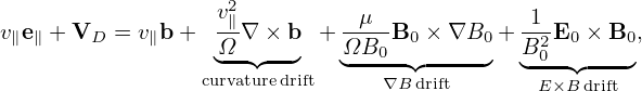
Using B∥0⋆ ≈ B0, then expression (385) is written as
| (388) |
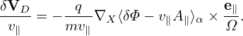
where the curvature drift, ∇B drift, and E0 × B0 drift can be identified. Note that the perturbed guiding-center velocity δVD is given by (refer to Sec. C.3)
| (389) |
Using the above results, equation (383) is written as
![[ ∂ ∂ ] ∂δf
∂t +(v∥e∥ + VD + δVD )⋅∂X-′ δf − e∥ ⋅μ ∇B0 ∂v
( ) ( ) ∥( )
= − δVD ⋅ ∂F0- + e∥-×∇X-⟨δϕ⟩α + v∥⟨δB-⊥⟩α- ⋅ μ-∇B0 ∂F0-
∂X ′ B0 B0 v∥ ∂v∥
q [ ∂⟨v ⋅δA ⟩ ( v2 μ 1 ⟨δB ⟩ ) ] ∂F 1
− -- − -------α-− v∥e∥ + -∥∇ × b+ ---- B0 × ∇B0 + -2E0 × B0 + v∥---⊥-α- ⋅∇X ⟨δϕ ⟩α --0(390),
m ∂t Ω ΩB0 B0 B0 ∂v∥ v∥](nonlinear_gyrokinetic_equation452x.png)
Collecting coefficients before ∂F0∕∂v∥, we find that the two terms involving ∇B0 (terms in blue and red) cancel each other, yielding
This equation agrees with Eq. (8) in I. Holod’s 2009 pop paper (gyro-averaging is wrongly omitted in that paper) and W. Deng’s 2011 NF paper.
![[ ∂ ∂ ] μ∂B0 ∂δG0
∂t + (v∥e∥ + VD + δVD )⋅∂X-′ δG0 − (v∥e∥ + VD + δVD )⋅v-∂X--∂v--
( ) ∥ ∥
= − δVD ⋅ ∂F0-− μ-∂B0-∂F0- − -q ∂⟨δL-⟩α-∂F0-1-, (380)
∂X ′ v∥∂X ∂v∥ m ∂t ∂v∥ v∥](nonlinear_gyrokinetic_equation439x.png)
![[ ∂ ∂ ] ∂δf
--+ (v∥e∥ + VD + δVD )⋅---′ δf − e∥ ⋅μ∇B0----
∂t ( ) ∂X ∂v∥
= − δVD ⋅ ∂F0- + δVD ⋅μ ∇B0 ∂F0-1
∂X ′ ∂v∥v∥
q [ ∂⟨v⋅δA ⟩α ( ⟨δB⊥ ⟩α ) ] ∂F0 1
− m- − ----∂t---− v∥e∥ + VD + v∥-B0--- ⋅∇X ⟨δϕ⟩α ∂v∥v∥. (383)](nonlinear_gyrokinetic_equation442x.png)
![[ ]
∂- +(v∥e∥ + VD + δVD )⋅-∂-′ δf − e∥ ⋅μ ∇B0 ∂δf
∂t ( ) ∂X ∂v∥
= − δV ⋅ ∂F0-
D ∂X
[ ( v2 ) ]
+ q- m-v∥⟨δB⊥-⟩α-⋅(μ∇B0 )+ ∂⟨v-⋅δA-⟩α + v∥b+ ∥-∇ ×b + -12E0 × B0 + v∥⟨δB-⊥⟩α ⋅∇X ⟨δϕ ⟩α ∂F0(3191,)
m q B0 ∂t Ω B 0 B0 ∂v∥ v∥](nonlinear_gyrokinetic_equation453x.png)