3 δf form of Vlasov equation in guiding-center variables

3.1 Electromagnetic field perturbation

Since the definition of the guiding-center variables (X,𝜀,μ,α) involves the equilibrium fields B₀ and E₀, to further simplify Eq. (52), we need to separate electromagnetic field into equilibrium and perturbation parts. Writing the electromagnetic field as

(53)

and

(54)

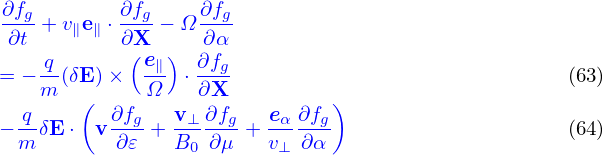
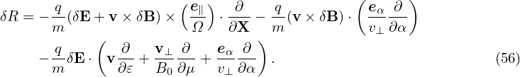
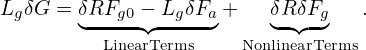
then substituting these expressions into equation (52) and moving all terms involving the field perturbations to the right-hand side, we obtain

where δR is defined by

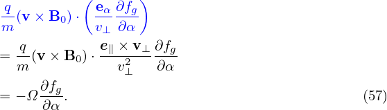
Next, let us simplify the left-hand side of Eq. (55). Note that

Note that

(58)

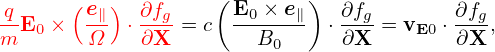
where v_E0 is defined by v_E0 = cE₀ × e_∥∕B₀, which is the E₀ × B₀ drift. Further note that

which can be combined with v ⋅ ∂f_g∕∂X term, yielding v_∥e_∥⋅ ∂f_g∕∂X.

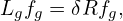
Using Eqs. (58),  (59), and  (57), the left-hand side of equation (55) is written as

where L_g is often called the unperturbed Vlasov propagator in guiding-center coordinates (X,𝜀,μ,α).

[Equation (60), corresponds to Eq. (7) in Frieman-Chen’s paper[3]. In Frieman-Chen’s equation (7), there is a term

where E_mac is a given macroscopic electric field introduced when defining the guiding-center transformation. In my derivation  E_mac is chosen to be equal to the equilibrium electric field, and thus the above term is zero.]

Using the above results, Eq. (55) is written as

(61)

i.e.

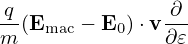
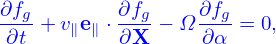
It is instructive to consider some special cases of the above complicated equation. Consider the case that the equilibrium magnetic field B₀ is uniform and time-independent, E₀ = 0, and the electrostatic limit δB = 0, then equation (62) is simplified as

If neglecting the δE perturbation, the above equation reduces to

(65)

which agrees with Eq. (21) discussed in Sec. 1.2.

3.2 Distribution function perturbation

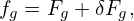
Expand the distribution function f_g as

(66)

where F_g is assumed to be an equilibrium distribution function, i.e.,

(67)

Using Eqs. (66) and (67) in Eq. (61), we obtain an equation for δF_g:

(68)

3.3 Gyrokinetic ordering

To facilitate the simplification of the Vlasov equation in the low-frequency regime, we assume the following orderings (some of which are roughly based on experiment measure of fluctuations responsible for tokamak plasma transport, some of which can be invalid in some interesting cases.) These ordering are often called the standard gyrokinetic orderings.

Assumptions for equilibrium quantities

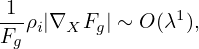
Define the spatial scale length L₀ of equilibrium quantities by L₀ ≈ F_g∕|∇_XF_g|. Assume that L₀ is much larger than the thermal gyro-radius ρ_i ≡ v_t∕Ω, i.e., λ ≡ ρ_i∕L₀ is a small parameter, where v_t = is the thermal velocity. That is

(69)

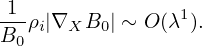
and

(70)

The equilibrium E₀ × B₀ flow, which is given by

(71)

is assumed to be weak with

(72)

Assumptions for perturbations

In terms of the scalar and vector potentials, δΦ and δA, the electromagnetic perturbation is written as

(73)

and

(74)

Most gyrokinetic simulations approximate the vector potential as δA ≈ δA_∥e_∥. Then Eq. (73) is writen as

(75)

We assume that the amplitudes of perturbations are small:

(76)

Further we assume that the parallel wavelength of perturbations is much longer than ρ_i:

(77)

and pependicular wavelength is of the same oder of ρ_i:

(78)

Equation (75) indicates that δB ∼ δA_∥∕ρ_i. Then the odering in (76) indicates that v_tδA_∥ is of the same order of δΦ.

The electrical field perturbation is written as

(79)

(80)

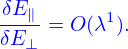
Using the above orderings, it is ready to see that δE_∥ is one order smaller than δE_⊥, i.e.,

(81)

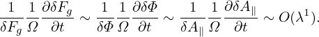
We assume the perturbations are of low frequency: ω∕Ω ∼ O(λ¹), i.e.,

(82)

3.4 Equation for macroscopic distribution function F_g

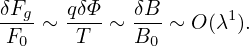
The evolution of the macroscopic quantity F_g is governed by Eq. (67), i.e.,

(83)

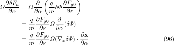
where the left-hand side is written as

Expand F_g as F_g = F_g0 + F_g1 + …., where F_gi ∼ F_g0O(λⁱ). Then, the balance on order O(λ⁰) gives

(84)

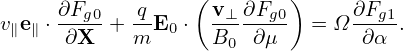
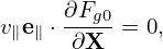
i.e., F_g0 is independent of the gyro-angle α. The balance on O(λ¹) gives

(85)

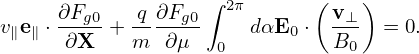
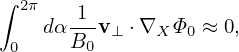
Performing averaging over α, ∫ ₀^2π(…)dα, on the above equation and noting that F_g0 is independent of α, we obtain

(86)

Note that a quantity A = A(x) that is independent of v will depend on v when transformed to guiding-center coordinates, i.e., A(x) = A_g(X,v). Therefore A_g depends on gyro-angle α. However, since ρ_i∕L ≪ 1 for equilibrium quantities, the gyro-angle dependence of the equilibrium quantities can be neglected. Specifically, e_∥, B₀ and Ω can be considered to be independent of α. As to v_∥, we have v_∥ = ±. Since B₀ is considered independent of α, so does v_∥. Using these results, equation (86) is written

(87)

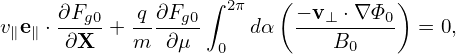
Using E₀ = −∇Φ₀, the above equation is written as

(88)

Note that

(89)

where the error is of O(λ²)Φ₀, and thus, accurate to O(λ), the last term of equation (88) is zero. Then equation (88) is written as

(90)

which implies that F_g0 is constant along a magnetic field line.

3.5 Equation for δF_g

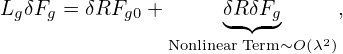
Using F_g ≈ F_g0, equation (68) is written as

(91)

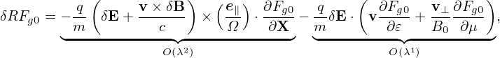
where δRδF_g is a nonlinear term which is of order O(λ²) or higher, L_gδF_g and δRF_g0 are linear terms which are of order O(λ¹) or higher. The linear term δRF_g0 is given by

(92)

In obtaining (92), use has been made of ∂F_g0∕∂α = 0. Another linear term L_gδF_g is written as

where Ω∂δF_g∕∂α is of order O(λ¹) and all the other terms are of order O(λ²).

Next, to reduce the complexity of algebra, we consider the easier case in which ∂F_g0∕∂μ = 0.

Balance on order O(λ¹): adiabatic response

The balance between the leading terms (terms of O(λ)) in Eq. (91) requires that

(94)

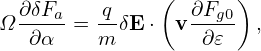
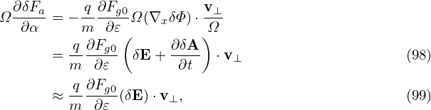
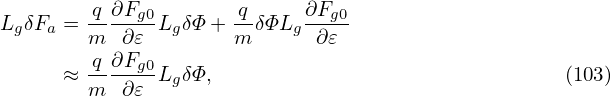
where δF_a is a unknown distribution function to be solved from the above equation. It is ready to verify that

(95)

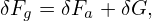
is a solution to the above equation, accurate to O(λ). [Proof: Substitute expression (95) into the left-hand side of Eq. (94), we obtain

Using

Eq. (96) is written as

where terms of O(λ²) have been dropped. Similarly, dropping the parallel electric field term (which is of O(λ²)) on the right-hand side of Eq. (94), we find it is identical to the right-hand side of Eq. (99)]

Separate δF_g into adiabatic and non-adiabatic part

As is discussed above, the terms of O(λ) can be eliminated by splitting a so-called adiabatic term form δF_g. Specifically, write δF_g as

(100)

where δF_a is given by (95), i.e.,

(101)

which depends on the gyro-angle via δΦ and this term is often called adiabatic term. Plugging expression (100) into equation (91), we obtain

(102)

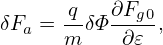
Next, let us simplify the linear term on the right-hand side, i.e, δRF_g0 −L_gfδF_a, (which should be of O(λ²) or higher because Ω∂δF_a∕∂α cancels all the O(λ¹) terms in δRF_g0).

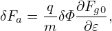
L_gδF_a is written

where the error is of order O(λ³). In obtaining the above expression, use has been made of e_∥⋅∂F_g0∕∂X = 0, ∂F_g0∕∂X = O(λ¹)F_g0, ∂F_g0∕∂α = 0, ∂F_g0∕∂μ = 0, and the definition of λ_B1 and λ_B2 given in expressions (39) and (40). The expression (103) involves δΦ operated by the Vlasov propagator L_g. Since δΦ takes the most simple form when expressed in particle coordinates (if in guiding-center coordinates, δΦ(x) = δΦ(X−v ×e_∥∕Ω), which depends on velocity coordinates and thus more complicated), it is convenient to use the Vlasov propagator L_g expressed in particle coordinates. Transforming L_g back to the particle coordinates, expression (103) is written

Using this and expression (92), δRF_g0 − L_gδF_a is written as

where the two terms of O(λ¹) (the terms in blue and red) cancel each other, with the remain terms being all of O(λ²), i.e, the contribution of the adiabatic term cancels the leading order terms of O(λ¹) on the RHS of Eq. (102).

The consequence of this is that, as we will see in Sec. 3.6.0, δG is independent of the gyro-angle, accurate to order O(λ¹). Therefore, separating δF into adiabatic and non-adiabatic parts also corresponds to separating δF into gyro-angle dependent and gyro-angle independent parts.

Linear term expressed in terms of δΦ and δA

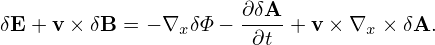
Let us rewrite the linear term (107) in terms of δΦ and δA. The δE + v ×δB term in expression (107) is written as

(108)

Note that this term needs to be accurate to only O(λ). Then

(109)

where the error is of O(λ²). Using the vector identity v ×∇_x ×δA = (∇δA) ⋅v − (v ⋅∇)δA and noting v is constant for ∇_x operator, the above equation is written

(110)

Note that Eq. (41) indicates that ∇_xδΦ ≈∇_XδΦ, where the error is of O(λ²), then the above equation is written

(111)

Further note that the parallel gradients in the above equation are of O(λ²) and thus can be dropped. Then expression (111) is written

where δL is defined by

(113)

Using expression (112), equation (107) is written

(114)

where all terms are of O(λ²).

3.6 Equation for the non-adiabatic part δG

Plugging expression (114) into Eq. (102), we obtain

(115)

where L_g is given by Eq. (93), i.e.,

Expansion of δG

Expand δG as

where δG_i ∼ O(λⁱ⁺¹)F_g0, and note that the right-hand side of Eq. (115) is of O(λ²), then, the balance on order O(λ¹) requires

(117)

i.e., δG₀ is gyro-phase independent.

The balance on order O(λ²) requires (for the special case of E₀ = 0):

Gyro-averaging

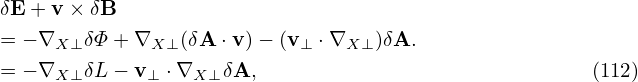
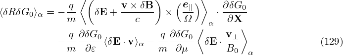
Define the gyro-average operator ⟨…⟩_α by

(119)

where h = h(X,α,𝜀,μ) is an arbitrary function of guiding-center variables. The gyro-averaging is an integration in the velocity space. [For a field quantity, which is independent of the velocity in particle coordinates, i.e., h = h(x), it is ready to see that the above averaging is a spatial averaging over a gyro-ring.]

Gyro-averaging Eq. (118), we obtain

where use has been made of ⟨(v_⊥⋅∇_X)δA⟩_α ≈ 0, where the error is of order higher than O(λ²). Note that v_∥ = ±. Since B₀ is approximately independent of α, so does v_∥. Using this, the first gyro-averaging on the left-hand side of the above equation is written

(121)

The second gyro-averaging on the left-hand side of Eq. (120) can be written as

(122)

where V_D is the magnetic curvature and gradient drift (Eq. (122) is derived in Appendix xx, to do later). Then Eq. (120) is written

Simplification of the nonlinear term

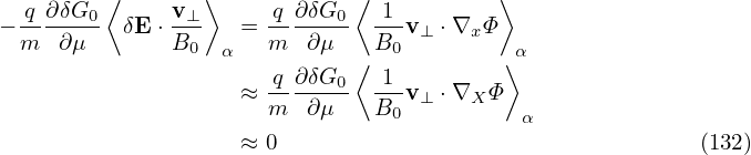
Next, we try to simplify the nonlinear term ⟨δRδF_g⟩_α appearing in Eq. (123), which is written as

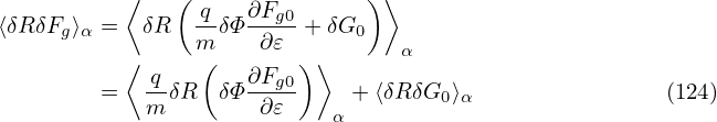
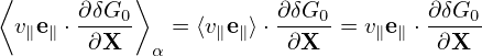
First, let us focus on the first term, which can be written as

Using the above results, the nonlinear term ⟨δRδF⟩_α is written as

(126)

Accurate to O(λ²),the first term on the right-hand side of the above is zero. [Proof:

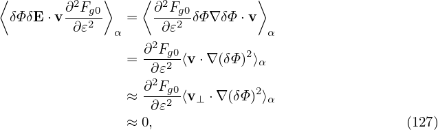
where use has been made of ⟨v_⊥⋅∇_XδΦ⟩_α ≈ 0, where the error is of O(λ²). Using the above results, expression (126) is written as

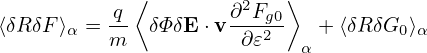
(128)

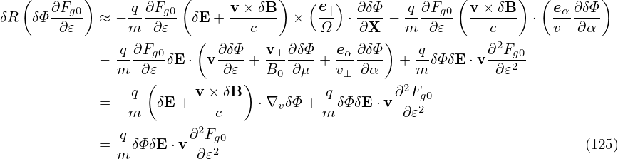
Using the expression of δR given by Eq. (56), the above expression is written as

where use has been made of ∂δG₀∕∂α = 0. Using Eq. (112), we obtain

(130)

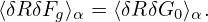
The other two terms in Eq. (129) can be proved to be zero. [Proof:

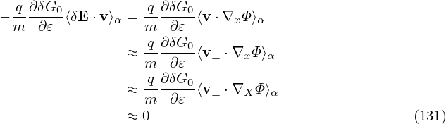
] Using the above results, the nonlinear term is finally written as

(133)

Using this in Eq. (128), we obtain

(134)

which is of O(λ²).

Final equation for the non-adiabatic part of distribution function perturbation

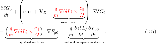
Using the above results, the gyro-averaged kinetic equation for δG₀ is finally written as

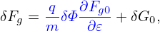
where δG₀ = δG₀(X,𝜀,μ,t) is gyro-angle independent and is related to the distribution function perturbation δF_g by

(136)

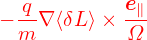
where the first term is called “adiabatic part”, which depends on the gyro-phase α via δΦ. (Equation (135) is the special case (∂F_g0∕∂μ|_𝜀 = 0) of the Frieman-Chen nonlinear gyrokinetic equation given in Ref. [3]. Note that the nonlinear terms only appear on the left-hand side of Eq. (135) and all the terms on the right-hand side are linear.) Here V_D is the guiding-center drift velocity in the equilibrim field; ⟨…⟩ is the gyro-phase averaging operator; δL = δΦ − v ⋅ δA; the term

(137)

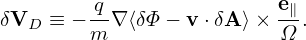
consists of the δE × B₀ drift and magnetic fluttering term (refer to  expression (341) in Sec. C.3). For notaiton ease, this term is denoted by δV_D in the following:

(138)

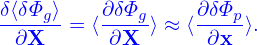
Note that ∇≡ ∂∕∂X, which is the gradient operator in the guiding-center coordinates (X,𝜀,μ,α) while holding (𝜀,μ,α) constant. How do we numerically calculate ∂Φ_g∕∂X in PIC simulations? The difficulty is that X grid is not available, which makes it difficult to use the finite difference method. Meanwhile x grid is available in PIC simulations. It turns out we can make use of x grid to approximatly calculate the derivatives in X space. Using x = X + ρ and the definition δΦ_g(X,α,v_⊥) = δΦ_p(x) we obtain

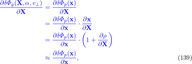
which is accurate up to O(λ) in gyrokinetic ordering. The above relation indicates that the value of ∂δΦ_g∕∂X at a guidng-center location is approximately equal to the value of ∂δΦ_p∕∂x at the corresponding particle position. Therefore we can use δΦ defined on x grid to compute  ∂δΦ_p∕∂x on gridpoints, and interpolate it to the particle position and this is a good approximation of ∂δΦ_g∕∂X.

Also note that ⟨δΦ_g⟩ is not known on X grid (it is known at random markers). So, to calculate ∂⟨δΦ_g⟩∕∂X, we need to exchange the operation order:

(140)

For notation ease, the subscripts g and p are usually dropped. Which one is intended should be obvious from the context.