4 Gyrokinetic equation suitable for numerical simulation

The gyrokinetic equation (135) contains time derivatives of unknown δΦ and δA on the right-hand side, which is problematic if treated by using explicit finite difference in PIC simulations. Next, we discuss some methods that can eliminate these terms, making the gyrokinetic equation more amenable to PIC simulations.

4.1 Eliminate ∂⟨δϕ⟩∕∂t term on the right-hand side of Eq. (135)

The coefficient before ∂F₀∕∂𝜀 in Eq. (135) involves the time derivative of ⟨δΦ⟩, which is problematic if treated by using explicit finite difference (I test the algorithm that treats this term by implicit scheme, the result roughly agrees with the standard method discussed in Sec. 5. In GEM’s split-weight scheme, ∂⟨δΦ⟩∕∂t is evaluated by using the vorticity equation (time derivative of the gyrokinetic Poisson equation).). It turns out that ∂⟨δΦ⟩∕∂t can be eliminated by defining another gyro-phase independent function δf by

(141)

Substituting this into Eq. (135), we obtain the equation for δf:

Noting that ∂F₀∕∂t = 0, e_∥⋅∇F₀ = 0, ∂F₀∕∂𝜀 ≈−F₀m∕T, we find that the third line of the above equation is of order O(λ³) (after both sides being divided by F₀Ω). Therefore the third line can be dropped. Moving the second line to the right-hand side and noting that ⟨δL⟩ = ⟨δΦ−v ⋅δA⟩, the above equation is written as

where two ∂⟨δΦ⟩∕∂t terms cancel each other. [Note that the right-hand side of Eq. (143) contains a nonlinear term δV_D ⋅∇_X⟨δΦ⟩. This is different from the original Frieman-Chen equation, where all nonlinear terms appear on the left-hand side. For the electrostatic limit, this term disappears because δV_D is perpendicular to ∇⟨δΦ⟩.]

Using

in the right-hand side of Eq. (143) yields

[Equation (144) corresponds to Eqs. (A8-A9) in Yang Chen’s paper[1], where the first minus on the right-hand side of Eq. (A8) is wrong and should be replaced with q∕m; one q is missing before ∂⟨v ⋅ δA⟩∕∂t in Eq. (A9).]

4.2 Eliminate ∂⟨v ⋅ δA⟩∕∂t term on the right-hand side of GK equation

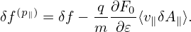
Similar to the method of eliminating ∂⟨δϕ⟩∕∂t, we define another gyro-phase independent function by

(145)

Most gyrokinetic simulations approximate the vector potential as δA ≈ δA_∥e_∥. Let us simplify Eq. (143) for this case. Then ⟨v ⋅ δA⟩ is written as

(146)

Then expression (145) is written as

(147)

Then Eq. (143) is written in terms of δf^(p_∥) as

where use has been made of that ∂F₀∕∂t = 0 and e_∥⋅∇F₀ = 0. Further noting that v_∥δA_∥∼ δΦ, qδΦ∕T ∼ O(λ¹), ∂F₀∕∂𝜀 ∼−F₀m∕T, V_D∕v_t ∼ O(λ¹), δV_D∕v_t ∼ O(λ¹), and ρ∇F₀ ∼ O(λ¹)F₀, we find that the red term of the above equation (after divided by ΩF₀) is of O(λ³), hence can be dropped. Move the second line to the right-hand side, giving

where ∂⟨v_∥δA_∥⟩∕∂t terms cancel each other. Further note that δV_D, given by Eq. (138), is perpendicular to ∇_X⟨δΦ − v_∥δA_∥⟩. Therefore the blue term in Eq. (149) is zero, then Eq. (149) simplifies to

Note that in terms of (X,𝜀,μ,α,σ) coordinates, v_∥ is written as

(151)

where B₀(x) = B₀(X + ρ) with ρ = ρ(X,𝜀,μ,α). Since the scale length of B₀ is much larger than the thermal Larmor radius, B₀(x) ≈ B₀(X) and hence v_∥ can be approximated as a constant when gyro-angle α changes. Then v_∥ can be taken out of the gyro-averaging in expression (146), yielding

(152)

Using this, the term related to δA_∥ in (150) can be further written as

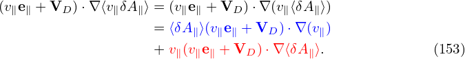
Using expression (151), ⟨δA_∥⟩(v_∥e_∥ + V_D) ⋅∇(v_∥) is written as

(We can also obtain ∇v_∥ = −μ(∇B₀)∕v_∥ by using Eq. (378).) Using the above results, equation (150) is written as

which agrees with the so-called p_∥ formulism given in the GEM manual (the first line of Eq. 28).

Besides the derivation given above, the equation can also be derived by using p_∥ = v_∥ + q⟨δA_∥⟩∕m as an independent variable (I did not verify this) and thus the name “p_∥ formulism”. There is another formulism called v_∥ formulism, which uses Eq. (144) as the gyrokinetic equation to be numerically solved. The difficulty of using v_∥ formulism is that the time derivative ∂A_∥∕∂t (in the weight evolution equation) needs to be treated by implicit schemes, otherwise it is numerical unstable[8]. On the other hand, the difficulty of using p_∥ formulism is that there is cancellation problems in Ampere’s law, as we will discuss in Sec. 4.7.

4.3 Summary of distribution function split

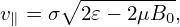
In the above, the total distribution function F is split as

(156)

where F₀ is the equilibrium distribution function and δF is the perturbation. Then δF is further split as

(157)

where δf^(p_∥) satisfies the gyrokinetic equation (155). In PIC simulations, δf^(p_∥) is evolved by using markers and its moment is evaluated via Monte-Carlo integration. The blue and red terms explicitly depends on the unknown perturbed field. After being integrated in the velocity space, these two terms give  the polarization density and the skin current, respectively. The polarization density is discussed in Sec. 5. The skin current is discussed in Sec. (4.4), and the so-called “cancellation problem” is discussed in Sec. 4.7.

4.4 Skin current

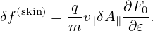
Let us calculate the moments of ⟨v_∥δA_∥⟩ (the blue term in Eq. (157)). Denote this term by δf^(skin). Neglect the FLR effect, then δf^(skin) is written as

(158)

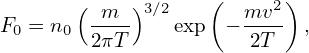
Assume that F₀ is a Maxwellian distribution:

(159)

then = −F₀, and expression (158) is written as

(160)

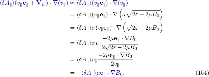
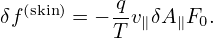
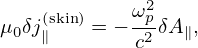
The number density carried by δf^(skin) is zero. The parallel current carried by δf^(skin) is given by

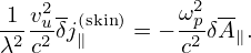
Working in the spherical coordinates, then v_∥ = v cos𝜃 and dv = v² sin𝜃dvd𝜃dϕ. Then expression (161) is written as

Using c = 1∕ and ω_p² = n ₀q²∕(m𝜀 ₀), the above expression can be written as

(163)

where the c∕ω_p is called “skin depth” and thus this current is often called “skin current” (some authors call it “adiabatic current”). We note the skin current is inversely proportional to the particle mass. So it is contributed mainly by electrons.

Gyrokinetic simulations indicate that the skin current δj_∥e^(skin) is often much larger than the actual δj_∥e. This means that δj_∥e^(skin) nearly cancels the current carried by δf_e^(p_∥), giving a small net current. This raises the question of whether numerical cancellation error is significant. It turns out that this error is indeed significant, which gives rise to numerical instabilities if no special treatment is used.

In TEK units:

(164)

(since

)

4.5 Mixed-variable pullback method

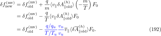
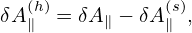
To mitigate the skin current cancellation problem, Mishchenko et al[7] introduced the “mixed-variable pullback” method. In this method, we define δA_∥^(h) by

(165)

with δA_∥^(s) determined by an evolution equation (inspired by the ideal Ohm’s law):

(166)

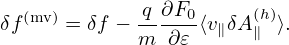
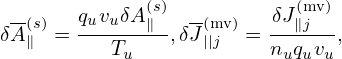
Using δA_∥^(h), we define a new distribution function δf^(mv) by

(167)

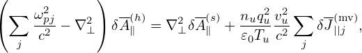
Then, starting from Eq. (143) and following the same procedure as that of Sec. 4.2, we obtain an equation for δf^(mv):

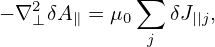
Meanwhile, the parallel Ampere equation

(169)

is written as

(170)

where δA_∥^(h) is the unknown to solve for, δJ_||j^(mv) is the parallel current carried by δf_j^(mv), where the subscript j is species index. Note that δA_∥^(s) has been moved to the rhs because its value is already known, by solving Eq. (166), before we solve the Ampere equation for δA_∥^(h).

In the above, a part of δA_∥ is solved from an evolution equation and the remainder is solved from the Ampere’s law. Can this scheme help to reduce numerical error? If A_∥^(s) carries the dominant part of δA_∥, then δA_∥^(h) will be small, then the skin current δA_∥^(h)ω_p²∕c² will be small, implying that the cancellation error will be small.

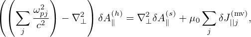
How do we ensure A_∥^(s) carry the dominant part of δA_∥ over the entire simulation duration? In addition to a careful choice of the evolution equation for δA_∥^(s), we have another leverage that can help δA_∥^(s) to remain dominant: collect the whole δA_∥ into δA_∥^(s) at the end of each time step:

(171)

Then, to make δA_∥ untouched (so that electromagnetic field remain unchanged), we set δA_∥^(h) to zero:

(172)

Here “old” and “new” refers to before and after the re-spliting, respectively. (This re-spliting is made at the end of each time step and does not correspond to any time evolution.) The re-splitting keeps the value of δA_∥ untouched and hence does not influence the electromagnetic field. Meanwhile, we need to keep δf unchanged. The definition of Eq. (167) indicates that, for a given δf, the re-splitting will make the value of δf^(mv) change to

(173)

This is the new initial value for δf^(mv). After this, the physical state of the system remains unchanged. This scheme makes δA_∥^(h) remain small for each time step mainly because δA_∥^(s) are set to carry all the value of δA_∥ at the begining of each time step. It is reasonable to assume that the variation of δA_∥ in a small time interval Δt is small. Denote this variation by Δ. In the best scenario, this small varaition will be captured by δA_∥^(s) if its evlution equation is chosen wisely. In the worst scenario, the time evolution of δA_∥^(s) may requires larger variation (than Δ) to be imposed on δA_∥^(h). Even in this senario,  δA_∥^(h) is still of order of Δ, which is the varation of δA_∥ in a small time step and hence small.

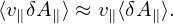
Next, consider the special case that F_g0 is local Maxwellian:

(174)

which is not an exact solution to the kinetic equation because X is not a constant of motion. We note that the radial coordinate of the guiding-center positon is approximately a constant of motion if the drift orbit width is small. So we restrict F_g0 to depending only on ψ, i.e.,

(175)

Then it is straightforward to calculate ∂F_g0∕∂𝜀 and ∇F_g0:

(176)

and

where κ_n ≡−, κ_T ≡−.

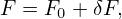
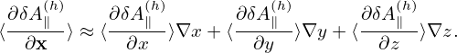
Using the above results, Eq. (168) is written as

where use has been made of ∇⟨δΦ⟩ = ⟨∇δΦ⟩ and ∇⟨δA_∥^(h)⟩ = ⟨∇δA_∥^(h)⟩.

In field-aligned coordinates

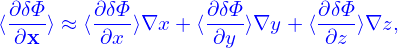
In field-aligned coordinates (x,y,z) (where x = ψ, y = α, z = 𝜃),  ∂δΦ∕∂x can be written as

(179)

Note that the direction of ∂r∕∂x at 𝜃 = −π is different from that at 𝜃 = +π. Therefore the value of ∂δΦ∕∂x at 𝜃 = −π is different from that at 𝜃 = +π. I.e., ∂δΦ∕∂x is a non-periodic function of 𝜃. Similarly, ∇y is also a non-perioidic functon of 𝜃. In other words, both ∂δΦ∕∂x and ∇y are discontinuous across the 𝜃 cut (𝜃 = ±π).

The gyro-average of expression (179) is written as

(180)

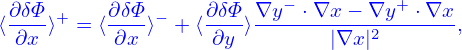
where we approximate ∇x, ∇y, and ∇z as constants when performing the gyro-averge since they are determined by the equilibrim magnetic field, which is nearly constant on the Larmor radius scale. As is mentioned above, ∇y is not continuous at the 𝜃 cut. Do we need to worry about this? No. This is because we must stick to the same branch when we perform gryo-average on it, and hence ∇y is always continous. Then, do we need to worry about the disconunity of ∂δΦ∕∂x across the 𝜃 cut when performing the gyro-averge on it? We do not either. The reason is the same: we must stick to a single branch. The disconunity is just irrelevant here. The discontinuity only manifest itself when we need to infer value on 𝜃 = +π from that on 𝜃 = −π (vice versa), i.e., when across branch communication is explicitly needed. In TEK, the field equations are not solved at 𝜃 = +π and hence the field values are not directly obtained. Instead, the field values at 𝜃 = +π are infered from the field values at 𝜃 = −π. At the 𝜃 cut and for the same (x,ϕ), the continuity of ∇δΦ requires

(181)

where the superscript “+” and “−” refer to the location 𝜃 = +π and 𝜃 = −π, respectively. Dotting the above by ∇x, we obtain

(182)

which is used in TEK to infer the value of ⟨⟩⁺ from that of ⟨⟩⁻.

Similarly,

(183)

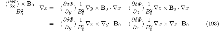
Then Eq. (178) is written as

where ≡ v_∥b + V_D + δV_D and ≡ V_D + δV_D. Define

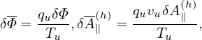
(185)

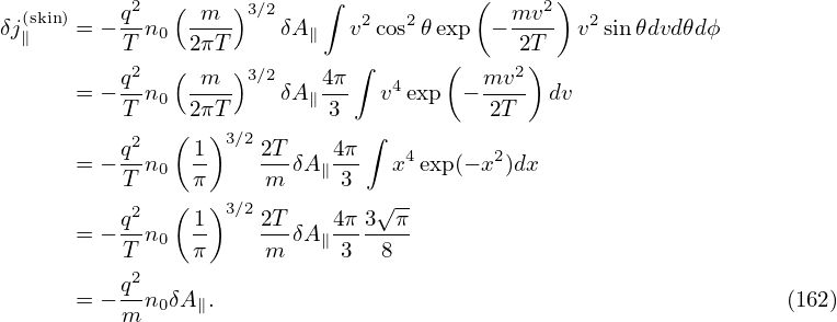
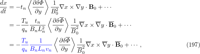
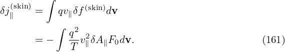
where q_u,T_u,v_u are units (independent of species), then Eq. (184) is written as

_____________________________________________________________________________________________Normalized Ampere’s equation__________________________________________________________________________________________________________________

Define

(188)

then Ampere equation (170) is written as

(189)

where use has been made of μ₀ = 1∕(c²𝜀₀).

__________________________________________________________________________________________________________________A_∥^(s) evolution_________________________________________________________________________________________________________________

In terms of units used in TEK, Eq. (166) is written as

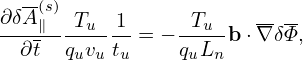
where t = t∕t_u with t_u = L_n∕v_u. The equation can be simplified as

(190)

i.e.,

(191)

____________________________________pullback_________________________________________________________

The pullback in Eq. (173) is now written as (for the case of F₀ being Maxwellian):

____________________________________________________________________________________________________________Perturbed drfit _______________________________________________________________________________________________________________________

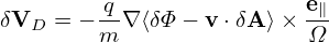
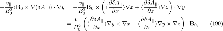
The δE × B₀ drift term is written as

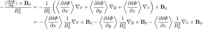
The ∇x, ∇y, and ∇z components of the above expression are written as

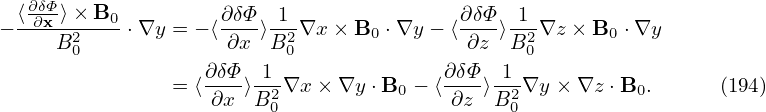
Note the general form:

(196)

Then, to get the normalizing factor, consider a typical term of the δE × B₀ drift:

where T_u∕(q_uv_nB_nL_n) is the normlizing factor we need when coding (in drift.f90).

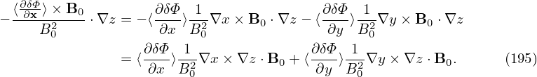
Next, consider the magnetic fluttering term, which is written as

The ∇x, ∇y, and ∇z components of the above expression are written as

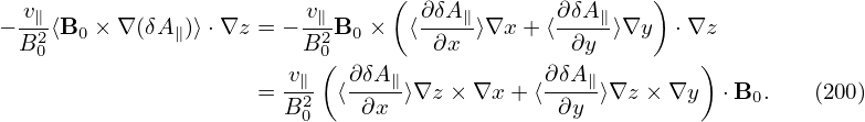
Also to get the normalizing factor, consider a typical term:

where T_u∕(q_uv_uB_nL_n) is the normlizing factor I need when coding (in drift.f90).

The equilibrium terms in the above can be written as

(202)

(203)

where the last entries in each lines are the variable names in TEK code.

4.6 Discretizing Laplacian operator

In TEK, the Laplacian operator is approximated as

(205)

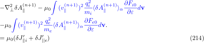
which is called “high-n approximation”, in which all derivatives with respect to z are dropped. This approximation reduces the Laplacian differential operator from 3D to 2D.

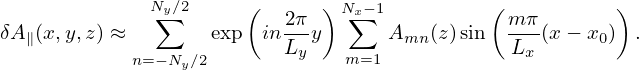
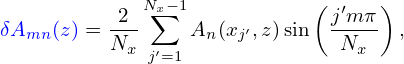
We assume that δA_∥ satisfies the zero boundary condition in the x direction: A_∥(x = x₀) = 0,A_∥(x = x₀ + L_x) = 0. Then the sine expansion can be used in this direction. In the y direction, full Fourier expansion is needed. I.e., at each value of z, A_∥(x,y,z) is approximated by the following two-dimensional expansion:

(206)

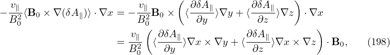
Use this expression, then −∇_⊥²δA_∥ of Eq. (205) is written as

At x = x_j, with x_j = x₀ + jΔ and L_x∕Δ = N_x, the above expression is written as

where ∇x and ∇y are evaluated at x_j. Plugging the DST coefficients

(208)

into expression (207) gives

For a single toroidal harmonic, the above expression reduces to

Define

then expression (209) is written as

(210)

4.7 Parallel Ampere’s Law in GEM code

(211)

where the parallel currents are given by

(212)

(213)

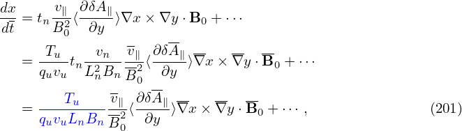
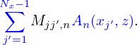
where δJ_∥i′ and δJ_∥e′ is the parallel current carried by the distribution function δf^(p_∥), which are updated from the value at the nth time step using an explicit scheme and therefore does not depends on the field at the (n + 1)th step. The blue terms  in Eqs. (212) and (213) are the “skin current”, which explicitly depend on the unknown field at the (n + 1)th step. If we want to solve Ampere’s law (211) by direct methods, then the blude terms need to be moved to the left-hand side. In this case, equation (211) is written as

Then we need to put the blue terms into matrix form. If we put the bule terms into martrix form by using numerical grid integration (as we do for the polarization density), then there arises the cancellation propblem (i.e., the two parts of the distribution are evaluated by different methods, one is grid-based and the other is MC marker based, there is a risk that the sum of the two terms will be inaccurate when the two terms are of opposite signs and large amplitudes, and the final result amplitude is expected to be much smaller than the amplituded of the two terms). If we get the matrix form by evaluating it numerically using MC markers (which can avoid the cancellation problem), the corresponding matrix will depends on markers and thus needs to be re-constructed each time-step, which is computationally expensive.

Therefore we go back to Eq. (211) and try to solve it using iterative methods. However, it is found numerically that directly using Eq. (211) as an iterative scheme is usually divergent. To obtain a convergent iterative scheme, we need to have an approximate form for the blue terms (bigger terms), which is independent of markers and so that it is easy to construct its matrix, and then subtract this approximate form from both sides. After doing this, the iterative scheme has better chance to be convergent (partially due to that the right-hand side becomes smaller). An approximate form is that derived by neglecting the FLR effect given in Sec. 4.4. Using this, the iterative scheme for solving Eq. (211) is written as

In the drift-kinetic limit (i.e., neglecting the FLR effect), the blue and red terms on the right-hand side of the above equation cancel each other exactly. Even in this case, it is found numerically that these terms need to be retained and the blue terms are evaluated using markers. Otherwise, numerical inaccuracy can give numerical instabilities, which is the so-called cancellation problem. The explanation for this is as follows. The blue terms are part of the current. The remained part of the current carried by δh is computed by using Monte-Carlo integration over markers. If the blue terms are evaluated analytically, rather than using Monte-Carlo integration over markers, then the cancellation between this analytical part and Monte-Carlo part can have large error (assume that there are two large contribution that have opposite signs in the two parts) because the two parts are evaluated using different methods and thus have different accuracy, which makes the cancellation less accurate.

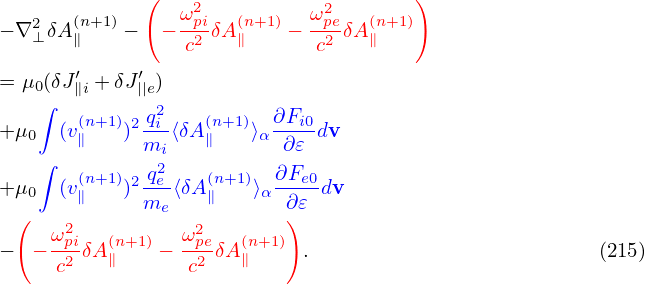
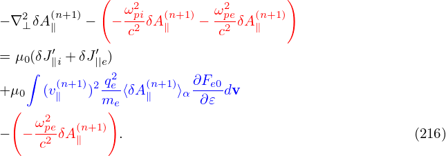
Because the ion skin current is smaller than its electron counterpart by a factor of m_e∕m_i, its accuracy is not important. The cancellation error for ions is not a problem and hence can be neglected. In this case, equation (215) is simplified as

Note that the blue term will be evaluated using Monte-Carlo markers.

4.8 Split-weight scheme for electrons in GEM code

The perturbed distribution function is decomposed as given by Eq. (157), i.e.,

(217)

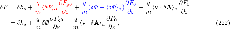
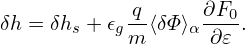
where the term in blue is the so-called adiabatic response, which depends on the gyro-angle in guiding-center coordinates. Recall that the red term ⟨δΦ⟩_α, which is independent of the gyro-angle, is introduced in order to eliminate the time derivative ∂⟨δΦ⟩_α∕∂t term on the right-hand side of the original Frieman-Chen gyrokinetic equation.

The so-called generalized split-weight scheme corresponds to going back to the original Frieman-Chen gyrokinetic equation by introducing another ⟨δΦ⟩_α term with a free small parameter 𝜖_g. Specifically, δh in the above is split as

(218)

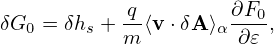
(If 𝜀_g = 1, then the two ⟨δΦ⟩_α terms in Eq. (217) and (218) cancel each other.) Substituting this expression into Eq. (), we obtain the following equation for δh_s:

Noting that ∂F₀∕∂t = 0, e_∥⋅∇F₀ = 0, ∇F₀ ∼ O(λ¹)F₀, we find that the third line of the above equation is of order O(λ³) and thus can be dropped. Moving the second line to the right-hand side, the above equation is written as

special case of 𝜖_g = 1

For the special case of 𝜖_g = 1 (the default and most used case in GEM code, Yang Chen said 𝜖_g < 1 cases are sometimes not accurate, so he gave up using it since 2009), equation (220) can be simplified as:

where two V_G ⋅⟨δΦ⟩_α terms cancel each other. Because the v_∥E_∥ term is one of the factors that make kinetic electron simulations difficult, eliminating V_G ⋅⟨δΦ⟩_α term may be beneficial for obtaining stable algorithms.

For 𝜖_g = 1, δF is written as

where the adiabatic term will be moved to the left-hand side of the Poisson’s equation. The descretization of this term is much easier than the polarization density.

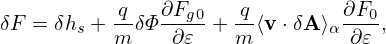
Equation (221) actually goes back to the original Frieman-Chen equation. The only difference is that ⟨v ⋅ δA⟩_α is split from the perturbed distribution function. Considering this, equation (221) can also be obtained from the original Frieman-Chen equation (135) by writing δG₀ as

(223)

In this case, δF is written as

(224)

Substituting expression (223) into equation (135), we obtain the following equation for δh_s:

Noting that ∂F₀∕∂t = 0, e_∥⋅∇F₀ = 0, ∇F₀ ∼ O(λ¹)F₀, we find that the third line of the above equation is of order O(λ³) and thus can be dropped. Moving the second line to the right-hand side, the above equation is written as

which agrees with Eq. (221).

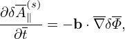
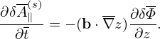
In GEM, the split weight method is used only for electrons. When using this scheme, ∂δΦ∕∂t appears on the right-hand-side of the weight evolution equation. GEM makes use of the vorticity equation (time derivative of the Poissson equation) to evaluate ∂δΦ∕∂t.