Fourier transformation in time

A general perturbation can be written

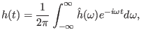$$h (t) = \frac{1}{2 \pi} \int_{- \infty}^{\infty} \hat{h} (\omega) e^{- i \omega t} d \omega,$$ (31)

where the coefficient $\hat{h} (\omega)$ is given by the Fourier transformation of $h (t)$, i.e.,

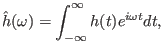$$\hat{h} (\omega) = \int_{- \infty}^{\infty} h (t) e^{i \omega t} d t,$$ (32)

Using the definition of the Fourier transformtion, it is ready to prove that

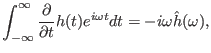$$\int_{- \infty}^{\infty} \frac{\partial}{\partial t} h (t) e^{i \omega t} d t = - i \omega \hat{h} (\omega),$$ (33)

and

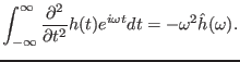$$\int_{- \infty}^{\infty} \frac{\partial^2}{\partial t^2} h (t) e^{i \omega t} d t = - \omega^2 \hat{h} (\omega) .$$ (34)

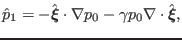
Performing Fourier transformation (in time) on both sides of the the linearized momentum equation (30) and noting that the equilibrium quantities are all independent of time, we obtain

$$- \omega^2 \rho_0 \hat{\ensuremath{\boldsymbol{\xi}}} = - \nabla ... ...B}_0 +{\textmu}_0^{- 1} (\nabla \times \mathbf{B}_0) \times \hat{\mathbf{B}}_1,$$ (35)

where use has been made of the property in Eq. (34). Similarly, the Fourier transformation of the equations of state (29) is written

$$\hat{p}_1 = - \hat{\ensuremath{\boldsymbol{\xi}}} \cdot \nabla p_0 - \gamma p_0 \nabla \cdot \hat{\ensuremath{\boldsymbol{\xi}}},$$ (36)

and the Fourier transformation of Faraday's law (28) is written

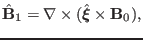$$\hat{\mathbf{B}}_1 = \nabla \times (\hat{\ensuremath{\boldsymbol{\xi}}} \times \mathbf{B}_0),$$ (37)

Equations (35)-(37) agree with Eqs. (12)-(14) in Cheng's paper[3]. They constitute a closed set of equations for $\hat{\ensuremath{\boldsymbol{\xi}}}$, $\hat{\mathbf{B}}_1$, and $\hat{p}_1$. In the next section, for notation ease, the hat on $\hat{\ensuremath{\boldsymbol{\xi}}}$, $\hat{\mathbf{B}}_1$, and $\hat{p}_1$ will be omitted, with the understanding that they are the Fourier transformations of the corresponding quantities.