
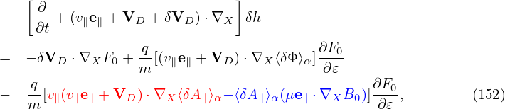
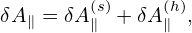
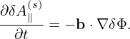
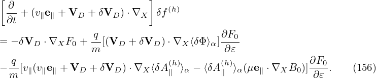
In the above, the perturbed part of the distribution function, δF, is split at least three times in order to (1) simplify the gyrokinetic equation by splitting out the adiabatic response and (2) eliminate the time derivatives, ∂δϕ∕∂t and (3) ∂δA∕∂t, on the right-hand. To avoid confusion, I summarize the split of the distribution function here. The total distribution function F is split as
|
| (150) |
where F0 is the equilibrium distribution function and δF is the perturbed part of the total distribution function. δF is further split as
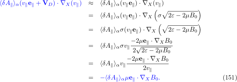 | (151) |
where δh satisfies the gyrokinetic equation (142) or (149). In Eq. (151), the red term gives rise to the so-called polarization density (discussed in Sec. 5.6). The analytic dependence of this term on δΦ is utilized in solving the Poisson equation. The blue term also has an analytic dependence on δA, which, however, will cause numerical problems in particle simulations if it is utilized in solving the Ampere equation (the so-called “cancellation problem” in gyrokinetic simulations).
 ⟨v ⋅ δA⟩α
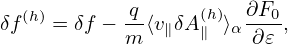
Consider the approximation δA ≈ δA∥e∥, then the blue term in Eq. (151) is written as
 | (152) |
Notice that v∥ can be taken out of the gyro-averaging. Then the above equation is written
 | (153) |
If we neglect the FLR effect, then the above expression is written
 | (154) |
The zeroth order moment (number density) is then written as
 | (155) |
which is zero if F0 is Maxwellian.
Next, consider the parallel current carried by distribution (154), which is written
 | (156) |
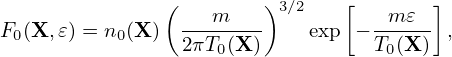
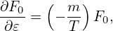
If F0 is a Maxwellian distribution given by
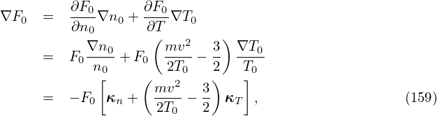 | (157) |
then
 | (158) |
Then expression (156) is written
 | (159) |
Working in the spherical coordinates, then v∥ = v cos𝜃 and dv = v2 sin𝜃dvd𝜃dϕ. Then expression (159) is written

 | (162) |
The parallel currents are given by
 | (163) |
 | (164) |
where δJ∥i′ and δJ∥e′ is the parallel current carried by the distribution function δh in Eq. (151), which are updated from the value at the nth time step to the (n + 1)th time step using an explicit scheme and therefore does not depends on the field at the (n + 1)th step. The blue terms in Eqs. (163) and (164) depend on the field at the (n + 1)th step and thus need to be moved to the left-hand side of Ampere’s law (162) if we want to solve this equation by direct methods. In this case, equation (162) is written as
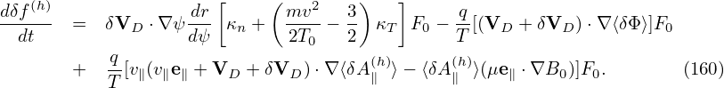
The blue terms are sometimes called “adiabatic current”. The red terms are approximation to the “adiabatic current” obtained by neglecting the FLR effect. Because the ion adiabatic current is less than the electron adiabatic current by a factor of me∕mi, its accuracy is not important, and is approximated by the drift-kinetic limit in GEM. And the cancellation error is not a problem and hence can be neglected. In this case, equation (166) is simplified as
![( )
− ∇2 δA(n+1) − μ − q2in δA(n+1) − q2en δA(n+1)
⊥ ∥ 0 mi i0 ∥ me e0 ∥
= μ [δJ′(δϕ(n),δA(n))+ δJ′(δϕ(n),δA (n))]
0∫ ∥i ∥ ||e ∥
+ μ (v(n+1))2-qi2⟨δA(n+1)⟩ ∂Fi0dv
0 ∥ mi ∥ α ∂𝜀
∫ (n+1)2-q2e (n+1) ∂Fe0
+ μ0 (v∥ )me ⟨δA∥ ⟩α ∂𝜀 dv
( q2 q2 )
− μ0 − -ini0δA(∥n+1)− -e-ne0δA (n∥+1) . (166)
mi me](nonlinear_gyrokinetic_equation175x.png)
![( )
− ∇2 δA(n+1) − μ − q2in δA(n+1) − q2en δA(n+1)
⊥ ∥ 0 mi i0 ∥ me e0 ∥
= μ [δJ′(δϕ(n),δA(n))+ δJ′(δϕ(n),δA (n))]
0∫ ∥i ∥ ||e ∥
+ μ (v(n+1))2 q2e⟨δA(n+1)⟩ ∂Fe0dv
0 ∥ me ∥ α ∂𝜀
( q2e- (n+1))
− μ0 − me ne0δA ∥ . (167)](nonlinear_gyrokinetic_equation176x.png)