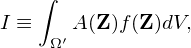
Consider a general integration of the distribution function f in the phase-space
|
| (53) |
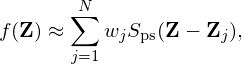
where Ω′ is a sub-region of the phase space Ω, A(Z) is a general function of the phase-space coordinates Z, dV is the phase space volume element. As is discussed above, in particle methods, f(Z) is approximated by
 | (54) |
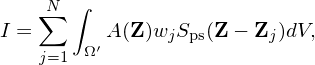
where Sps(Z−Zj) is the phase space shape function of markers, N is the total number of marker loaded in the phase space Ω. Using this, expression (53) is written as
 | (55) |
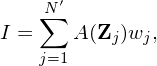
If the shape function Sps is chosen to be the Dirac delta function, then the above equation is written as
 | (56) |
where N′ is the number of markers that are within the sub-region Ω′. Equation (56) is the Monte-Carlo approximation to the integration in Eq. (53)[4, 2].
In PIC simulations, we are usually interested in velocity moments of f averaged in a cell, i.e., A in Eq. (55) is only a function of only v and the velocity integration is over the whole velocity space, whereas the spatial integration is over a small spatial cell. Furthermore, in PIC simulations, the markers are assumed to have a finite shape in the real space (the shape in velocity space is still the Dirac delta function). In this case, Eq. (55) is written as
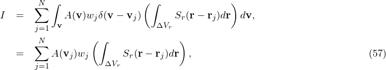
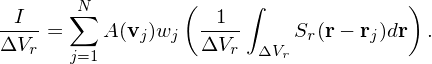 | (58) |