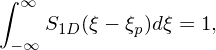
A marker (super-particle) in PIC simulations represents a group of physical particles, which has their own distribution function given by
|
| (22) |
where the subscript p denotes quantities on a marker, wp is the weight of the marker defined above, Sv(v − vp) and S(r − rp) are the shape functions in the velocity space and real space, respectively. Here Sv and S have physical diemsion of 1∕length3 and 1∕velocity 3 so that the physical dimension of fp given in expression (22) is consistent with the physical dimension of a distribution function.
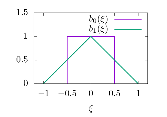
In standard PIC simulation, the shape of markers in the velocity space is always a Dirac delta function:
 | (23) |
where δ3(v − vp) is the three-dimensional Dirac delta function. In this case, all the physical particles represnted by a marker have the same veloicty vp. [In terms of general velocity coordinates (vα,vβ,vγ), the three-dimensional Dirac delta function is defined via the 1D Dirac delta function as follows:
 | (24) |
where 𝒥 is the the Jacobian of the general velocity coordinate system (vα,vβ,vγ). Note that 𝒥v is dimensionless and the 1D Dirac delta function δ(vα − vαp) has a physical dimension of 1∕vα.]
The shape function in the real space, S(r − rp), can also be chosen as the Dirac delta function. In practice, finite-size shape in spatial space is often adopted, i.e., the physical particles represented by a marker have different spatial locations. Along with the cell-averaging (discussed later), finite-size shape function has the effect of making the resulting self-consistent field more smooth, reducing (ideally completely removing) the artificial collision effects (the interaction among close particles) associated with using very few markers to approximate a plasma that has many physical particles in a Debye sphere[7].
A 3D shape function can be constructed by combining three 1D shape functions and the Jacobian of the coordinate system. For example, in (α,β,γ) coordinate system, a 3D shape function is written as
![1 [ 1 ( α − α )] [ 1 ( β − β ) ][ 1 (γ − γ )]
S (r − rp) = --- ----S1D -----p ----S1D ----p- ----S1D -----p ,
𝒥r Δαp Δαp Δβp Δβp Δ γp Δ γp](particle_simulation24x.png) | (25) |
where 𝒥r = 𝒥r(α,β,γ) is the Jacobian of (α,β,γ) coordinate system, Δαp, Δβp, and Δγp are the scale-lengths of the support of the 1D shape function S1D along α, β, and γ directions, respectively. The 1D shape function S1D should satisfy the following normalization:
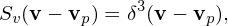
 | (26) |
where ξ is one of the spatial coordinates. The reason to include the Jacobian in the definition of the 3D shape function is that this makes fp be consistent with the definition of a distribution function, i.e., satisfy the following normalization:
 | (27) |
i.e.,
 | (28) |
While not strictly necessary, symmetric shapes are usually chosen, i.e. S1D has the property: S1D(ξ −ξp) = S1D(ξp −ξ). The support of S1D should be compact (i.e. it is zero outside a small region) so that physical particles represnted by the marker are localized to a small portion of the space. Compact support of S1D can make the deposition and gathering operations (defined later) computationally efficient. Modern PIC codes usually use the so-called b-splines as the spatial shape functions. The b-spline functions are a series of consecutively higher order functions obtained from each other by integration:
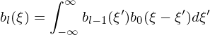 | (29) |
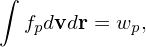
with the 0th b-spline being the flat-top function defined as
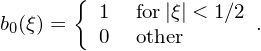 | (30) |
Then, by using Eqs. (29) and (30), it is ready to derive the expression of b1(ξ), which is given by
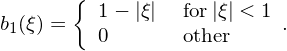 | (31) |
The graphics of the first two b-splines, b0(ξ) and b1(ξ), are shown in Fig. 1.
The 1D shape function based on the b-spline function is then given by
 | (32) |
Most PIC codes use b0, i.e, the flat-top function, as the shape function and choose the support of the shape function Δp equal to the grid spacing. (k-spectra of particle shape functions, to be continued)
The shape functions are essentially identical to the basis functions used in finite element methods.
The spatial shape of markers determines how physical particles represented by a marker are distributed to spatial cells (called deposition) and also how the force on a marker is related to the nearby electromagnetic field. Note that the phase-space volume occupied (or sampled) by a marker is different from the concept of the spatial-shape of a marker.
The physical particle distribution is the sum of all the particle elements given in expression (22), i.e.,
 | (33) |