Finite difference form of toroidal elliptic operator in general coordinate system

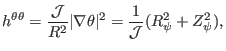
The toroidal elliptic operator in Eq. (415) can be written

$$\triangle^{\ast} \Psi = \frac{R^2}{\mathcal{J}} [(h^{\psi \psi} \... ...^{\psi \theta} \Psi_{\theta})_{\psi} + (h^{\psi \theta} \Psi_{\psi})_{\theta}],$$ (422)

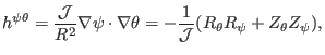
where $h^{a \beta}$ is defined by Eq. (174), i.e.,

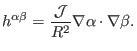$$h^{\alpha \beta} = \frac{\mathcal{J}}{R^2} \nabla \alpha \cdot \nabla \beta .$$ (423)

Next, we derive the finite difference form of the toroidal elliptic operator. The finite difference form of the term $(h^{\psi \psi} \Psi_{\psi})_{\psi}$ is written

$$(h^{\psi \psi} \Psi_{\psi})_{\psi} \vert _{i, j} = \frac{1}{\delta \psi} \left[ h^{\psi \psi}_{i, j + 1 / 2} \left( ... ... \psi} \left( \frac{\Psi_{i, j} - \Psi_{i, j - 1}}{\delta \psi} \right) \right]$$

$$= H^{\psi \psi}_{i, j + 1 / 2} (\Psi_{i, j + 1} - \Psi_{i, j}) - H^{\psi \psi}_{i, j - 1 / 2} (\Psi_{i, j} - \Psi_{i, j - 1}),$$ (424)

where

$$H^{\psi \psi} = \frac{h^{\psi \psi}}{(\delta \psi)^2} .$$ (425)

The finite difference form of $(h^{\theta \theta} \Psi_{\theta})_{\theta}$ is written

$$(h^{\theta \theta} \Psi_{\theta})_{\theta} \vert _{i, j} = \frac{1}{\delta \theta} \left[ h^{\theta \theta}_{i + 1 / 2, j} \... ..., j} \left( \frac{\Psi_{i, j} - \Psi_{i - 1, j}}{\delta \theta} \right) \right]$$

$$= H^{\theta \theta}_{i + 1 / 2, j} (\Psi_{i + 1, j} - \Psi_{i, j}) - H^{\theta \theta}_{i - 1 / 2, j} (\Psi_{i, j} - \Psi_{i - 1, j}),$$ (426)

where

$$H^{\theta \theta} = \frac{h^{\theta \theta}}{(\delta \theta)^2} .$$ (427)

The finite difference form of $(h^{\psi \theta} \Psi_{\theta})_{\psi}$ is written as

$$\left.(\Psi_{\theta} h^{\psi \theta})_{\psi} \right\vert _{i, j} ... ...i + 1, j - 1 / 2} - \Psi_{i - 1, j - 1 / 2}}{2 \delta \theta} \right) \right] .$$ (428)

Approximating the value of $\Psi$ at the grid centers by the average of the value of $\Psi$ at the neighbor grid points, Eq. (428) is written as

$$(\Psi_{\theta} h^{\psi \theta})_{\psi} \vert _{i, j} = H^{\psi \t... ...Psi_{i + 1, j - 1} + \Psi_{i + 1, j} - \Psi_{i - 1, j - 1} - \Psi_{i - 1, j}) .$$ (429)

where

$$H^{\psi \theta} = \frac{h^{\psi \theta}}{4 \delta \psi d \theta} .$$ (430)

Similarly, the finite difference form of $(h^{\psi \theta} \Psi_{\psi})_{\theta}$ is written as

$$(\Psi_{\psi} h^{\psi \theta})_{\theta} \vert _{i, j} = \frac{1}{\delta \theta} \left[ h^{\psi \theta}_{i + 1 / 2, j} \le... ...si_{i - 1 / 2, j + 1} - \Psi_{i - 1 / 2, j - 1}}{2 \delta \psi} \right) \right]$$

$$= H^{\psi \theta}_{i + 1 / 2, j} (\Psi_{i + 1, j + 1} + \Psi_{i, j ... ...Psi_{i, j + 1} + \Psi_{i - 1, j + 1} - \Psi_{i, j - 1} - \Psi_{i - 1, j - 1}) .$$ (431)

Using the above results, the finite difference form of the operator $\mathcal{J} \triangle^{\star} \Psi / R^2$ is written as

$$\left. \frac{\mathcal{J}}{R^2} \triangle^{\ast} \Psi \right\vert _{i, j} = (h^{\psi \theta} \Psi_{\theta})_{\psi} + (h^{\psi \psi} \Psi_{\ps... ...\theta \theta} \Psi_{\theta})_{\theta} + (h^{\psi \theta} \Psi_{\psi})_{\theta}$$

$$= H^{\psi \psi}_{i, j + 1 / 2} (\Psi_{i, j + 1} - \Psi_{i, j}) - H^{\psi \psi}_{i, j - 1 / 2} (\Psi_{i, j} - \Psi_{i, j - 1})$$

$$+ H^{\theta \theta}_{i + 1 / 2, j} (\Psi_{i + 1, j} - \Psi_{i, j}) - H^{\theta \theta}_{i - 1 / 2, j} (\Psi_{i, j} - \Psi_{i - 1, j})$$

$$+ H^{\psi \theta}_{i, j + 1 / 2} (\Psi_{i + 1, j} + \Psi_{i + 1, j ... ...(\Psi_{i + 1, j - 1} + \Psi_{i + 1, j} - \Psi_{i - 1, j - 1} - \Psi_{i - 1, j})$$

$$+ H^{\psi \theta}_{i + 1 / 2, j} (\Psi_{i + 1, j + 1} + \Psi_{i, j ... ...(\Psi_{i, j + 1} + \Psi_{i - 1, j + 1} - \Psi_{i - 1, j - 1} - \Psi_{i, j - 1})$$

$$= \Psi_{i, j} (- H^{\psi \psi}_{i, j + 1 / 2} - H^{\psi \psi}_{i, j - 1 / 2} - H^{\theta \theta}_{i + 1 / 2, j} - H^{\theta \theta}_{i - 1 / 2, j})$$

$$+ \Psi_{i - 1, j - 1} (H^{\psi \theta}_{i, j - 1 / 2} + H^{\psi \th... ..., j - 1 / 2} - H^{\psi \theta}_{i + 1 / 2, j} + H^{\psi \theta}_{i - 1 / 2, j})$$

$$+ \Psi_{i + 1, j - 1} (- H^{\psi \theta}_{i, j - 1 / 2} - H^{\psi \... ... - 1 / 2, j} - H^{\psi \theta}_{i, j + 1 / 2} + H^{\psi \theta}_{i, j - 1 / 2})$$

$$+ \Psi_{i + 1, j} (H^{\theta \theta}_{i + 1 / 2, j} + H^{\psi \thet... ...- 1, j + 1} (- H^{\psi \theta}_{i, j + 1 / 2} - H^{\psi \theta}_{i - 1 / 2, j})$$

$$+ \Psi_{i, j + 1} (H^{\psi \psi}_{i, j + 1 / 2} + H^{\psi \theta}_{... ...i + 1, j + 1} (H^{\psi \theta}_{i, j + 1 / 2} + H^{\psi \theta}_{i + 1 / 2, j})$$

The coefficients are given by

$$h^{\psi \psi} = \frac{\mathcal{J}}{R^2} \vert \nabla \psi \vert^2 = \frac{1}{\mathcal{J}} (R_{\theta}^2 + Z_{\theta}^2),$$ (432)

$$h^{\theta \theta} = \frac{\mathcal{J}}{R^2} \vert \nabla \theta \vert^2 = \frac{1}{\mathcal{J}} (R_{\psi}^2 + Z_{\psi}^2),$$ (433)

and

$$h^{\psi \theta} = \frac{\mathcal{J}}{R^2} \nabla \psi \cdot \nabla \theta = - \frac{1}{\mathcal{J}} (R_{\theta} R_{\psi} + Z_{\theta} Z_{\psi}),$$ (434)

where the Jacobian

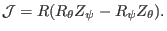$$\mathcal{J}= R (R_{\theta} Z_{\psi} - R_{\psi} Z_{\theta}) .$$ (435)

The partial derivatives, $R_{\theta}$, $R_{\psi}$, $Z_{\theta}$, and $Z_{\psi}$, appearing in Eqs. (432)-(435) are calculated by using the central difference scheme. The values of $h^{\psi \psi}$, $h^{\theta \theta}$, $h^{\psi \theta}$ and $\mathcal{J}$ at the middle points are approximated by the linear average of their values at the neighbor grid points.

dd